Statelets: Capturing recurrent transient variations in dynamic functional network connectivity

Abstract

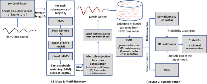
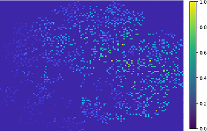
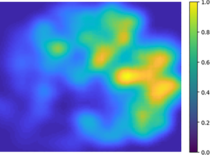
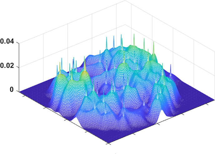
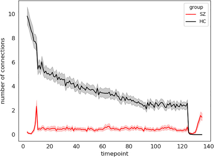
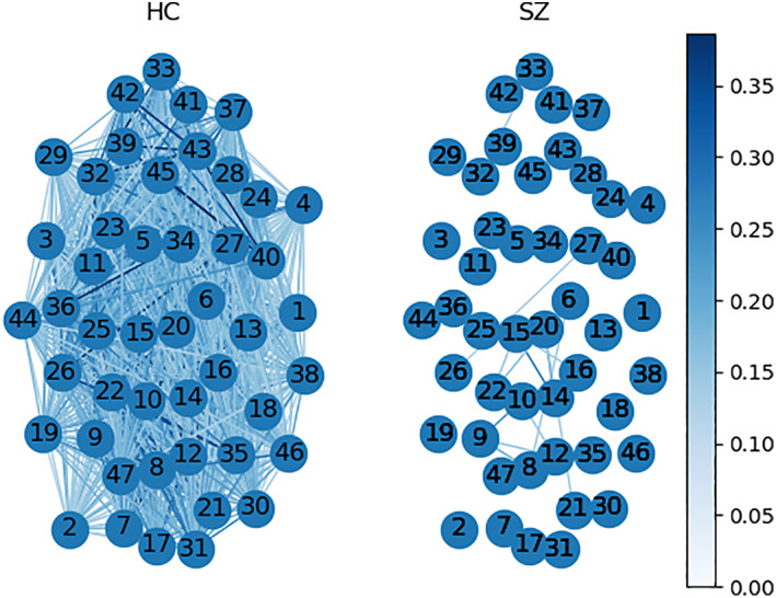
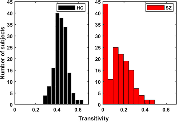
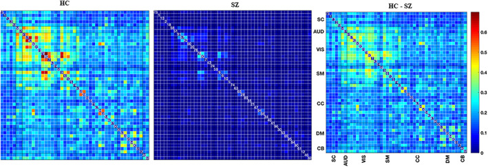
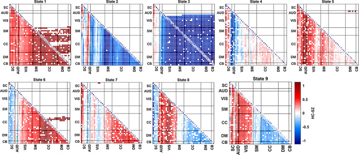
Dynamic functional network connectivity (dFNC) analysis is a widely used approach for capturing brain activation patterns, connectivity states, and network organization. However, a typical sliding window plus clustering (SWC) approach for analyzing dFNC models the system through a fixed sequence of connectivity states. SWC assumes connectivity patterns span throughout the brain, but they are relatively spatially constrained and temporally short-lived in practice. Thus, SWC is neither designed to capture transient dynamic changes nor heterogeneity across subjects/time. We propose a state-space time series summarization framework called "statelets" to address these shortcomings. It models functional connectivity dynamics at fine-grained timescales, adapting time series motifs to changes in connectivity strength, and constructs a concise yet informative representation of the original data that conveys easily comprehensible information about the phenotypes. We leverage the earth mover distance in a nonstandard way to handle scale differences and utilize kernel density estimation to build a probability density profile for local motifs. We apply the framework to study dFNC of patients with schizophrenia (SZ) and healthy control (HC). Results demonstrate SZ subjects exhibit reduced modularity in their brain network organization relative to HC. Statelets in the HC group show an increased recurrence across the dFNC time-course compared to the SZ. Analyzing the consistency of the connections across time reveals significant differences within visual, sensorimotor, and default mode regions where HC subjects show higher consistency than SZ. The introduced approach also enables handling dynamic information in cross-modal and multimodal applications to study healthy and disordered brains.

Keywords: dynamic functional network connectivity; earthmover distance; kernel density estimator; resting-state MRI; schizophrenia; time series motifs summarization.

FIGURE 1

Our proposed methodology for time series motifs discovery and summarization. (a) Step 1: Motif extraction using EMD as a similarity metric. The subroutine takes out the most repetitive pattern (possibly with multiple occurrences) of a given time course, (b) Step 2: Summarization of motifs using their probability density computed by a kernel density estimator (KDE). It takes a bag of varying length motifs and generates a concise smaller collection of the most frequent shapes/patterns representing the functional system (SZ/HC). We defined these prototypes as the statelets. The EMD distance matrix is used for both performing the tSNE and computing probability density (PD) of the motifs. The relevant processing blocks and their intuitions in Step 2 are described elaborately in Section 5.2

FIGURE 2

An example of tSNE using EMD distance on a collection of real motifs. Data points represent the motifs weighted by their probability density computed using KDE. X and Y axis stand for the horizontal and vertical coordinates of each point, respectively

FIGURE 3

Mapping tSNE points to a 2D matrix for accumulating PD's of close neighbors. Therefore, we observe the higher density data with a brighter color in the figure

FIGURE 4

After applying a Gaussian blur on the 2D image to defocus less dense data points

FIGURE 5

A three‐dimensional view of the tSNE plot after marking the peaks extracted by a 2D peak finder. The peak finder selects at least one peak from each high‐density region. Later, we use peak's tSNE coordinates to determine the real motifs it represents

FIGURE 6

A subset of dominant motifs from SZ and HC dynamics. The motifs are detrended and visualized using tSNE followed by the Jonker‐Volgenant algorithm for the linear assignment problems. A similar type of shape is embedded into the same neighborhood. We can see a few potential subgroups of motifs. The blank space in the figure was generated because we used a larger 2D grid than the number of motifs to display. So, the algorithm optimizes the location for each motif from the 2D coordinate system to assign the matching patterns in the nearby vicinity. The X axis is time, and the Y axis represents the dynamic functional connectivity strength

FIGURE 7

Each connection's probability density (PD) demonstrates how frequently the statelets extracted from a connection appear in the group dynamic. Each connection has two density values: one per subject group. Blue demonstrates PD in controls (HC) and red in the patients (SZ). We sort the connections low to high according to their PD in the SZ group (left subplot), and HC sorts the right subplot. Y axis represents the order of the links after sorting, and X axis depicts their corresponding PD. We observe that the rank of connections differs in both subject's groups in terms of their PD; the PD difference is statistically significant and visually evident in the plot

FIGURE 8

Each graph represents the occurrences of the most recurring statelets over each subject's time course. These are three randomly selected subjects from the HC (top) and SZ (bottom) groups. We convolve the group statelets with the subject dynamics (all the dFNC time courses, 1,081) to investigate the recurrence of the statelets over time. Then, we sorted the pairs based on the dominant shape's first occurrence in their time series. Consequently, the early the statelets appear in a pair's time course, the higher the pair/connection in that subject's dynamics—we threshold these convolutions matching scores at 0.8 for both groups to track down the strong appearances only. The color intensity corresponds to how strongly/weakly the shape appears in that part of the course. The color bar is identical for all the reference subjects in the figure

FIGURE 9

Based on probability density ranking (in Figure 7), we computed a collective appearance of the connections across all the subjects. The X axis shows the time steps, and the Y axis corresponds to the number of pairs connections that show the first statelet at that step, which indicates the activation of the pair

FIGURE 10

Time decay graphs from both groups. The nodes are functional networks, edges correspond to the connection between them (maximum 1,081 possible), and the weight represents the mean time decay (TD) of a connection within a group dynamic. We compute color scaling from the 95 percentiles of the total values. After thresholding at average group mean (SZ group mean + HC group mean)/2, 1,061 edges survive in the HC group and only 16 edges in the SZ group

FIGURE 11

Histogram of transitivity from subject‐wise time decay graphs. It refers to the extent to which the relation between two nodes in a network connected by an edge is transitive. A significant portion of SZ subjects shows 0 transitivity, which means the connections are less consistent across different subjects. We show the differences are statistically significant using a two‐sample t‐test on both distributions. Transitivity is also related to the clustering coefficient

FIGURE 12

Pairwise mean time decays in healthy control (HC) and schizophrenia (SZ) groups. We run a two sample t test on the pairwise time decay values to check the statistical significance of their HC‐SZ group differences. The rightmost subfigure represents the FDR corrected t values

FIGURE 13

Classification accuracy for different methods. First, three methods were applied to the dFNC matrix and LSTM with the attention model applied to the dFNC time course. The last two methods use time decay (TD) for classification. We run the models on time decay information of all the subjects for 100 repeated iterations, and the accuracies are mean across the iterations. We train the model on 200 random samples in each iteration and cross‐validate them using the remaining 114 subjects

FIGURE 14

HC—SZ group differences in terms of max connectivity strength. State‐wise group differences in functional connectivity (FC). We have both SZ and HC subjects' groups at each state. For each pair of components, we have a subset of statelets from HC subjects and a subset from SZ subjects. Then, we compute the maximum connectivity strength of those statelets from both subgroups. A two‐sample t test using a null hypothesis of “No group difference” compares patients' max connectivity versus controls. A higher t value indicates the rejection of the null hypothesis irrespective of their sign. However, the sign of t values represents the directionality of the group difference. The pair matrix (47 × 47) is labeled into seven different domains subcortical (SB), auditory (AUD), visual (VIS), sensorimotor (SM), cognitive control (CC), defaultmode (DM), cerebellar (CB), respectively. White cells in the matrix indicate either the absence of that pair or nonsignificant group differences for this pair within a state. The upper triangle represents the FDR corrected differences

References

1. Agcaoglu, O. , Wilson, T. W. , Wang, Y. P. , Stephen, J. M. , & Calhoun, V. D. (2020). Dynamic resting‐state connectivity differences in eyes open versus eyes closed conditions. Brain Connectivity, 10(9), 504–519. - PMC - PubMed
1. Ahmad, I. A. , & Amezziane, M. (2007). A general and fast convergent bandwidth selection method of kernel estimator. Journal of Nonparametric Statistics, 19(4–5), 165–187.
1. Ahmad, S. , Taskaya‐Temizel, T. , & Ahmad, K. (2004). Summarizing time series: Learning patterns in ‘volatile’ series. In International conference on intelligent data engineering and automated learning. Exeter, England: Springer.
1. Aine, C. J. , Bockholt, H. J. , Bustillo, J. R. , Cañive, J. M. , Caprihan, A. , Gasparovic, C. , … Calhoun, V. D. (2017). Multi‐modal neuroimaging in schizophrenia: Description and dissemination. Neuroinformatics, 15(4), 343–364. - PMC - PubMed
1. Alavash, M. , Tune, S. , & Obleser, J. (2019). Modular reconfiguration of an auditory control brain network supports adaptive listening behavior. Proceedings of the National Academy of Sciences, 116(2), 660–669. - PMC - PubMed
Publication types