The BrainScaleS-2 Accelerated Neuromorphic System With Hybrid Plasticity

Abstract

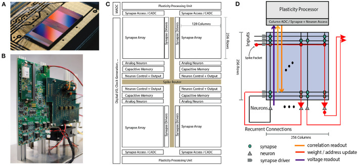
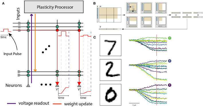
Since the beginning of information processing by electronic components, the nervous system has served as a metaphor for the organization of computational primitives. Brain-inspired computing today encompasses a class of approaches ranging from using novel nano-devices for computation to research into large-scale neuromorphic architectures, such as TrueNorth, SpiNNaker, BrainScaleS, Tianjic, and Loihi. While implementation details differ, spiking neural networks-sometimes referred to as the third generation of neural networks-are the common abstraction used to model computation with such systems. Here we describe the second generation of the BrainScaleS neuromorphic architecture, emphasizing applications enabled by this architecture. It combines a custom analog accelerator core supporting the accelerated physical emulation of bio-inspired spiking neural network primitives with a tightly coupled digital processor and a digital event-routing network.

Keywords: neuromorphic computing; neuroscientific modeling; physical modeling; plasticity; spiking neural network accelerator.

Figure 1

Overview of the BrainScaleS-2 System architecture. (A) Bonded chip on its carrier board, one can see the two synaptic crossbar arrays. (B) Test setup, with the chip (covered by white plastic) mounted on a carrier board. The Field Programmable Gate Array (FPGA) and I/O boards have been designed by our collaboration partners at TU Dresden. (C) Schematic floorplan of the chip: Two processor cores with access to the synaptic crossbar array are on the top and bottom. The 512 neuron circuits and analog parameter storage are arranged in the middle. The event router routes events generated by the neurons and external events to the synapse drivers and to/from the digital I/O located on the left edge of the chip. (D) Conceptual view of the system architecture in spike processing mode: Event packets (red dot) get injected by the synapse driver into the synaptic crossbar, where they cause synaptic input integration to occur in synapses with matching addresses (indicated by red lines). Membrane voltage accumulation eventually results in spike generation in the associated neuron circuits. The resulting spikes are routable to both synapse drivers or external output. The plasticity processing unit has low latency and massively parallel access to synaptic weights, addresses, correlation measurements, and neuron membrane voltage dynamics during operation. Plasticity rules and other learning algorithms can use these observables to modify all parameters determining network emulation in an online fashion.

Figure 2

Histograms showing a characterization of LIF properties of neurons before (top) and after (bottom) calibration. Each histogram shows all 512 neuron circuits on a single ASIC. In the top row, the configuration has been set equal for all neurons, to the median of the calibrated parameters. This results in different model characteristics due to device-specific fixed-pattern noise arising during the manufacturing process. After calibration, the analog parameters, such as bias currents and voltages, are selected such that the observed characteristics match a target.

Figure 3

Faithfully emulating the original AdEx equations, BrainScaleS-2's neuron circuits can be configured to generate distinct firing patterns as a response to a constant current stimulus. Here, we tuned the neuron circuits exemplarily to replicate four of the patterns described by Naud et al. (2008) using automated calibration routines. Each of the four panels features the time evolution of the membrane trace and the adaptation current, as well as the resulting trajectory through the phase space.

Figure 4

Emulating multi-compartmental neuron models on BrainScaleS-2. (A) Four compartments are connected to form a chain, compare model at the top and left side. The traces show the membrane potential in the four different compartments as a synaptic input is injected in one compartment after another. Thanks to the high configurability of the BrainScaleS-2 system, compare Section 2.2, the conductance between the individual compartments can be altered to control the attenuation of the signal along the chain. (B) Model of a chain which splits in two. The BrainScaleS-2 system supports dendritic spikes, here demonstrated in the form of plateau potentials. Inputs are injected in different compartments with a fixed delay between them; this is indicated by the vertical bars above the membrane traces. Depending on the spatio-temporal distribution of the inputs a dendritic spike can be elicited. The traces show the membrane potential in compartment 0. Figure adapted from Kaiser et al. (2021).

Figure 5

Insect-inspired path integration and navigation on the BrainScaleS-2 accelerated neuromorphic substrate. (A) Network activity and path during a single experiment instance. The simulated agent first randomly spreads out from the “nest” until it finds “food.” It then returns to the nest using the integrated path information. Once returned, it starts looping around the nest until the experiment is terminated. The blue lines indicate how points along the trajectory correspond to the activity trace shown below. From top to bottom, the neuron activity traces are that of the two sensory neurons (TN), “compass” neurons (TB), integrators (CPU4), steering (CPU1), and motor neurons (M). Signals flow from TN → TB, TB → CPU4, CPU1; CPU4 → CP1 and CP1 → M. Details of the network architecture were given by Schreiber (2021). (B) We performed evolutionary optimization of the weights controlling the behavior of our agents. Here we show 3 sample trajectories each of the initial (primeval) and evolved population. Inset is a histogram over 1.000 trajectories in the final “looping” phase of the evaluation, zoomed in to a 6.000 × 6.000 square of positions at the origin. As can be seen, the evolved population reaches a more symmetrical and tighter looping behavior. (C) Influence of two hyperparameters h, k on the integration performance of the spiking integrators, each 12.000 × 12 000 square of positions contains a histogram of 100 trajectories in the looping phase (t>2t_return) for a total of 4.200 trajectories. (D) Response to excitatory and inhibitory input rates of the calibrated CPU1 neurons. The dashed line indicates where 50 % of the maximum output rate is expected. Calibration of these neurons, as well as all the other neurons, was done on-chip using the PPU, in the case of the implementation done on the full-scale BrainScaleS-2 system. (A–D) are adapted from Schreiber (2021), (D) uses data from Leibfried (2021).

Figure 6

Real world closed loop interaction with the BrainScaleS-2 system. (A) Conceptual overview of the example experiment, a sensor head with three light sensors is moved over an illuminated surface. Sensor readings are converted into spike input to 3 input sources in a small feedforward spiking neural network. Spike output produced by 4 neurons is converted into motor commands, which move the sensor head on the surface. The goal is to follow the light gradient. (B) Physical realization of the example experiment from right to left: The PlayPen2 consists of two actuated arms which pantographically move a sensor head over a screen or illuminated surface. Signals from the sensor head are digitally processed by a micro controller and converted into spikes send into a FPGA used to interface with a scaled down BrainScaleS-2 prototype system, which implements the small feedforward spiking network. Spike outputs are routed in the FPGA to the Spike I/O interface and converted by pulse shapers into motor command pulses. (C) Example trajectories of the sensor head on the surface, with gray indicating the accessible region (left) and zoom in on the center region where the brightness maximum is (right). (E) Position (top) and brightness signals (bottom) of the sensor head over time. The two panels on the left show the full time course. The neural network starts control at t = 100 ms and stops at t = 250 ms. The two panels on the right show a zoom in on the interval t ∈ [100, 200]ms, with the gray curve indicating an average over all brightness readings. (D) We perform evolutionary optimization of the 4 × 3 weight matrix both from a random initial weight configuration. We show the moving average of the fitness in black and the fitness at a certain generation in gray, both for the top three individuals (dashed line) and the population average (solid line). In addition we display the weight configuration of an arbitrary individual at 6 selected generations (0, 3, 10, 25, 50, and 100). Finally we show a qualitative performance evaluation at the same generations of the average weight matrix over 100 experimental runs divided into 4 starting positions. The contourlines show where 99, 50, and 10% of all trajectories ended after 225 ms, when the maximum brightness should be reached. The contourlines are overlayed over a plot of the brightness sampled from the photo diode signals over all runs and generations. Missing pixels correspond to locations not reached at any time. (A–E) were adapted from Schreiber (2021) and (C) from Billaudelle et al. (2020).

Figure 7

Exploiting collective dynamics for information processing on BrainScaleS-2. (A) The autocorrelation time τ_ac of recurrent SNNs can be controlled by changing the input strength K_ext under the constant application of homeostatic regulation. (B) The emerging autocorrelation times for low K_ext can be exploited for complex, memory-intensive task processing. Both, a n bit sum as well as a n bit parity task profit from the complex processing capabilities for high n. Low n task, in contrast, profit from short time scales and hence high K_ext. The optimal K_ext for each n is highlighted by red stars. As a result, each task requires its own dynamic state. (C) The adaptation of the network dynamics to task requirements can be achieved by switching the input strength under the constant action of homeostatic regulation irrespective of the initial condition. Here, the transition from a state with long time scales to short ones is completed with only a few homeostatic weight updates (i). The reverse transition requires a longer relaxation phase (ii).

Figure 8

Training of and inference with SNNs on BrainScaleS-2 using surrogate gradients. (A) Exemplary activity snapshots for three 16 × 16 pixel MNIST images, the resulting spike-latency encodings, an overlay of the hidden layer membrane traces recorded at a data rate of 1.2 Gbit/s as well as the resulting hidden layer spikes, and the output layer membrane traces. (B) Spike-latency encoding promotes fast decision times: after 7 μs the network reaches its peak performance. (C) A fast inference mode allows to exploit the quick decision times by artificially resetting the neuronal states after 8 μs and therefore preparing the network for presentation of the next sample, culminating in a classification rate of 85 k inferences per second. (D) The PyTorch-based framework allows to co-optimize for near-arbitrary regularization terms, including sparsity penalties. In this instance, BrainScaleS-2 can be trained to classify MNIST images with an average of 12 hidden layer spikes per image without a significant decline in performance.

Figure 9

Use of the BrainScaleS-2 system in ANN operating mode. (A) Analog input values are represented as pulses sent consecutively into the synaptic crossbar. The duration of these pulses represents input activations. Synapses modulate the pulse height depending on the stored weight. Signed weights can be achieved by using two synapse rows, excitatory and inhibitory, for the same input. The neuron circuits serve as an integrator of the generated currents. Readout of the voltage occurs in parallel once triggered (dashed violet line) by the columnar ADC. (B) Layers that exceed the hardware resources are tiled into hardware execution instances and sequentially executed. Panel taken from Spilger et al. (2020). (C) Example membrane traces during inference of MNIST handwritten digits in the output layer. The ten output activations are sampled at the indicated time for all neurons in parallel.

Figure 10

(A) A large dynamical system consisting of two decoupled subsystems. It has a block diagonal Jacobian and corresponding decoupled sensitivity equations. (B) Parameter gradient computation in sequentially composed physical systems (orange) can be performed by composing gradient computation in models of the physical systems (blue).

References

1. Aamir S. A., Müller P., Kiene G., Kriener L., Stradmann Y., Grübl A., et al. . (2018a). A mixed-signal structured AdEx neuron for accelerated neuromorphic cores. IEEE Trans. Biomed. Circ. Syst. 12, 1027–1037. 10.1109/TBCAS.2018.2848203 - DOI - PubMed
1. Aamir S. A., Stradmann Y., Müller P., Pehle C., Hartel A., Grübl A., et al. . (2018b). An accelerated LIF neuronal network array for a large-scale mixed-signal neuromorphic architecture. IEEE Trans. Circ. Syst. 65, 4299–4312. 10.1109/TCSI.2018.2840718 - DOI
1. Barnett L., Lizier J. T., Harré M., Seth A. K., Bossomaier T. (2013). Information flow in a kinetic ising model peaks in the disordered phase. Phys. Rev. Lett. 111, 177203. 10.1103/PhysRevLett.111.177203 - DOI - PubMed
1. Barton P. I., Lee C. K. (2002). Modeling, simulation, sensitivity analysis, and optimization of hybrid systems. ACM Trans. Model. Comput. Simul. 12, 256–289. 10.1145/643120.643122 - DOI
1. Bellec G., Salaj D., Subramoney A., Legenstein R., Maass W. (2018). Long short-term memory and learning-to-learn in networks of spiking neurons. arXiv preprint arXiv:1803.09574.
LinkOut - more resources