Review
. 2022 Jun;48(6):975-996.
doi: 10.1016/j.ultrasmedbio.2022.01.009. Epub 2022 Mar 11.

Spatial Coherence in Medical Ultrasound: A Review

Affiliations
Review

Spatial Coherence in Medical Ultrasound: A Review

James Long et al. Ultrasound Med Biol. 2022 Jun.

Abstract

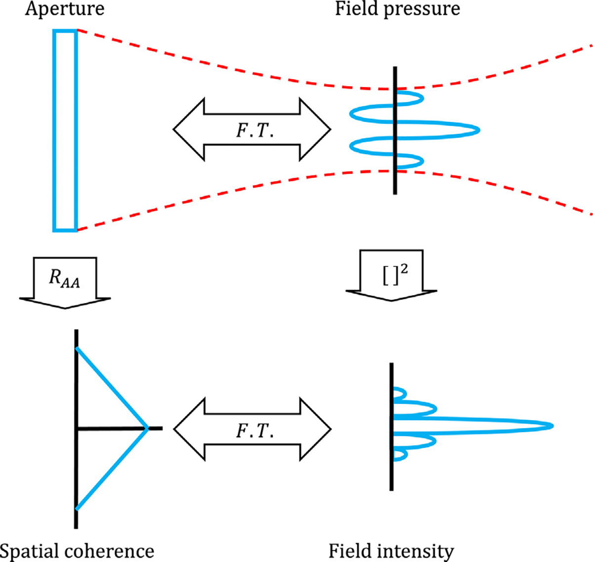
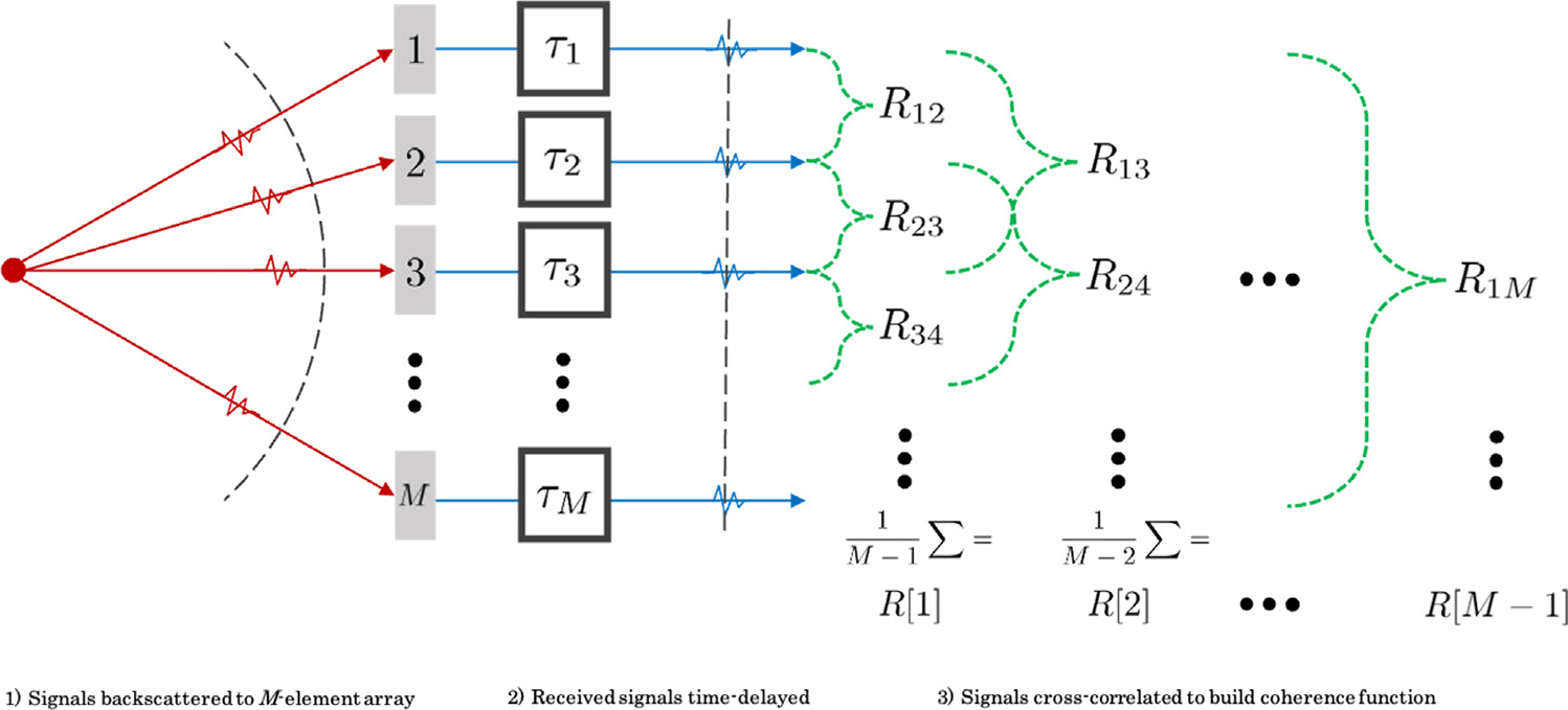
Traditional pulse-echo ultrasound imaging heavily relies on the discernment of signals based on their relative magnitudes but is limited in its ability to mitigate sources of image degradation, the most prevalent of which is acoustic clutter. Advances in computing power and data storage have made it possible for echo data to be alternatively analyzed through the lens of spatial coherence, a measure of the similarity of these signals received across an array. Spatial coherence is not currently explicitly calculated on diagnostic ultrasound scanners but a large number of studies indicate that it can be employed to describe image quality, to adaptively select system parameters and to improve imaging and target detection. With the additional insights provided by spatial coherence, it is poised to play a significant role in the future of medical ultrasound. This review details the theory of spatial coherence in pulse-echo ultrasound and key advances made over the last few decades since its introduction in the 1980s.

Keywords: Beamforming; Clutter reduction; Image quality characterization; Spatial coherence; Tissue characterization.


Figures

Fig. 1.
Fig. 1.
Fourier transform (F.T.) relationships between the aperture function, field intensity profile and spatial coherence function. The aperture, shown at the top left, is a rectangle function in this example.
Fig. 2.
Fig. 2.
Three-stage process for calculation of the coherence function. First, signals are backscattered to an M-element array (red). Second, time delays are applied to received signals (blue). Third, correlation pairs are calculated for each lag of the coherence function (green).
Fig. 3.
Fig. 3.
Propagation through fat and septa in a computerized human abdominal wall. Frames are shown 3.8 apart in time μs, and the area is 22.9 × 14.4 mm. Light blue regions of the abdominal wall correspond to fat; dark blue regions correspond to connective tissue. Reprinted, with permission, from Mast et al. (1997).
Fig. 4.
Fig. 4.
Transverse fetal abdomen acquisition at four different acoustic output levels, labeled with corresponding mechanical indices. Images are shown over a 70-dB dynamic range, and axes are in centimeters. Reprinted, with permission, from Flint et al. (2021). MI = mechanical index.
Fig. 5.
Fig. 5.
Illustration of the analytic spatial coherence function in the ideal, noise-free case (black) and in the presence of incoherent (blue) and partially coherent noise (red). Analytic calculation performed using the framework from Walker and Trahey (1997).
Fig. 6.
Fig. 6.
In vivo images of a cyst at a depth of 1.5 cm in a human thyroid: (a) B-mode, (c) short-lag spatial coherence at Q = 10.4%, (c) Q = 20.8%, (d) Q = 31.2% and (e) a spatially compounded image. All images are shown with a 50-dB dynamic range. Reprinted, with permission, from Lediju et al. (2011).
Fig. 7.
Fig. 7.
Tissue harmonic image (THI, left) and harmonic spatial coherence image (HSCI, right) of an apical two-chamber view for a cardiac patient. Reprinted, with permission, from Hyun et al. (2019).
Fig. 8.
Fig. 8.
Power Doppler (PD) images revealing a sagittal view of a neonatal brain cortex for (a) conventional PD and (b) short-lag angular coherence (SLAC) PD. PD images are shown as an overlay to the B-mode. Arrows indicate small vasculature discernible in SLAC PD, but not in conventional PD. Reprinted, with permission, from Jakovljevic et al. (2021).
Fig. 9.
Fig. 9.
Brachytherapy seed visualization with B-mode (a, d), delay and sum (DAS) photo-acoustic imaging (b, e) and short-lag spatial coherence (SLSC) photo-acoustic imaging (c, f), for linear (a–c) and curvilinear (d–f) arrays. Photo-acoustic images are shown as an overlay to the B-mode. Arrows and numbers in the B-mode indicate the position of visible seeds, and the urethra is indicated with green. Reprinted, with permission, from Bell et al. (2014).
Fig. 10.
Fig. 10.
Example fundamental and harmonic in vivo fetal images before (top) and after (bottom) lag-one spatial coherence adaptive normalization (LoSCAN). Contrast, contrast-to-noise ratio (CNR) and generalized CNR (gCNR) for regions of interest, indicated by dashed white lines, are reported in the bottom left of each image. Reprinted, with permission, from Long et al. (2020b).
Fig. 11
Fig. 11
. In vivo images of a breast carcinoma with microcalcifications. (a) High-frame-rate (HFR) B-mode image. (b) B-mode weighted with coherence factor adjusted for minimum variance beamforming (CFMV). (c) Original B-mode with a reduced dynamic range (DR) to match the speckle variance in (b). Microcalcifications are indicated with arrows in (c). Reprinted, with permission, from Wang and Li (2009).
Fig. 12.
Fig. 12.
Example in vivo images comparing (left to right) B-mode, receive spatial compounding, short-lag spatial coherence (SLSC) and multicovariate imaging of subresolution targets (MIST). Reprinted, with permission, from Morgan et al. (2019b).
Fig. 13.
Fig. 13.
Backscatter tensor imaging in a porcine myocardial sample, with the B-mode image (a) and measured coherence functions (b). Coherence functions across the fibers and along the fibers are in blue and red, respectively. Reprinted, with permission, from Papadacci et al. (2014).
Fig. 14.
Fig. 14.
Correlation maps in a healthy patient (a) and a patient with severe steatosis (b). The determined sound speed characterizing the medium is highlighted on the vertical axes. Reprinted, with permission, from Imbault et al. (2017).

Similar articles

Cited by

References

    1. Adler L, Hiedemann EA. Determination of the nonlinearity parameter B/A for water and m-xylene. J Acoust Soc Am 1962;34:410–412.
    1. Ahmed R, Bottenus N, Long J, Trahey GE. Reverberation clutter suppression using 2-D spatial coherence analysis. IEEE Trans Ultrason Ferroelectr Freq Control 2022;69:84–97. - PMC - PubMed
    1. Anderson ME, Soo MSC, Trahey GE. Microcalcifications as elastic scatterers under ultrasound. IEEE Trans Ultrason Ferroelectr Freq Control 1998;45:925–934. - PubMed
    1. Asl BM, Mahloojifar A. Minimum variance beamforming combined with adaptive coherence weighting applied to medical ultrasound imaging. IEEE Trans Ultrason Ferroelectr Freq Control 2009;56:1923–1931. - PubMed
    1. Bamber JC, Hill CR. Acoustic properties of normal and cancerous human liver-I. Dependence on pathological condition. Ultrasound Med Biol 1981;7:121–133. - PubMed

Publication types