Three-dimensional light-field microendoscopy with a GRIN lens array

Abstract

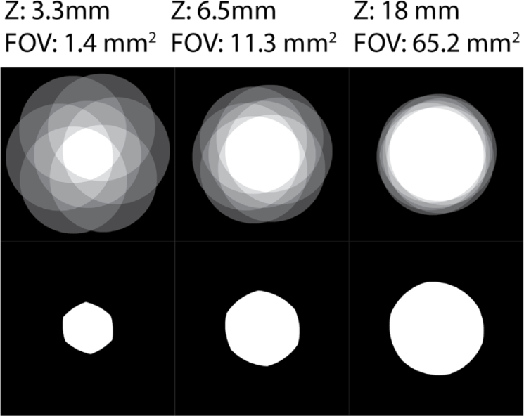
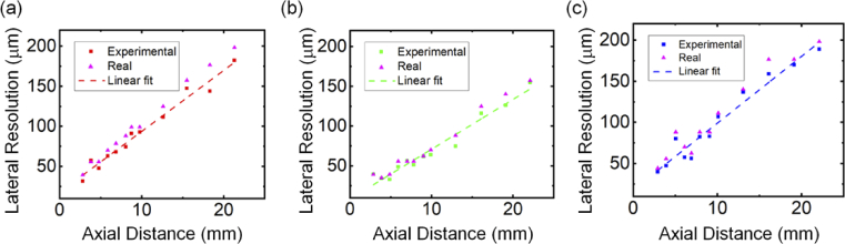
Optical endoscopy has emerged as an indispensable clinical tool for modern minimally invasive surgery. Most systems primarily capture a 2D projection of the 3D surgical field. Currently available 3D endoscopes can restore stereoscopic vision directly by projecting laterally shifted views of the operating field to each eye through 3D glasses. These tools provide surgeons with informative 3D visualizations, but they do not enable quantitative volumetric rendering of tissue. Therefore, advanced tools are desired to quantify tissue tomography for high precision microsurgery or medical robotics. Light-field imaging suggests itself as a promising solution to the challenge. The approach can capture both the spatial and angular information of optical signals, permitting the computational synthesis of the 3D volume of an object. In this work, we present GRIN lens array microendoscopy (GLAM), a single-shot, full-color, and quantitative 3D microendoscopy system. GLAM contains integrated fiber optics for illumination and a GRIN lens array to capture the reflected light field. The system exhibits a 3D resolution of ∼100 µm over an imaging depth of ∼22 mm and field of view up to 1 cm². GLAM maintains a small form factor consistent with the clinically desirable design, making the system readily translatable to a clinical prototype.

Fig. 1.

GRIN lens array microendoscopy (GLAM) design and image formation. (a) CAD model of the endoscope assembly. (b) Assembled endoscope system with overlaid dimensions of the insertion tube. Inset shows a close-up of the 3D printed core of the insertion tube that holds the seven GRIN lenses and six illumination fibers. (c) Schematic diagram of light propagation through the system. RL, doublet relay lenses.

Fig. 2.

Chromatic calibration of GLAM. (a) Schematic representation of axial chromatic aberration in the system. Inset shows laterally displaced RGB PSF positions in the off-axis elemental images. (b) Axial stack projection (step size = 50 µm) of the RGB PSF within an axial range of 22 mm. Inset shows the zoomed-in image of the yellow boxed region. The colors can be clearly resolved closer to GLAM, indicating an enhanced axial resolution. (c) Projection of the PSF shift from lens center for each elemental image along the y-z axis. A 0-10 mm axial displacement range is shown for better visualization of the point separation close to the endoscope. Scale bars: 20 µm (a), 500 µm (b), 50 µm (b, inset).

Fig. 3.

System characterization using M(z). (a) Magnification of RGB as a function of the distance of the object from the system. Solid lines show the average magnification for each color, and the shaded areas represent the standard deviation over all the lenses. (b) FOV, defined as the overlapping region of all seven lenses in the reconstruction. (c) The Nyquist sampling resolution limit of the system. (d) Axial resolution given as the smallest resolvable axial shift over distance.

Fig. 4.

Experimental system characterization. (a) Magnification of RGB as a function of distance from the system. Solid lines show the average magnification for each color, and the shaded areas represent the standard deviation over all the lenses. (b) Reconstructed RGB images of the USAF target taken at 2.85 mm away from GLAM. Inset shows the zoomed-in image of Group 4 (physical size: 535 µm × 1173 µm). (c) The black curve shows the overall intensity profile along the finest resolvable elements indicated by the red line in (b). The red, green, and blue curves represent the Gaussian-fitting of the three corresponding bars. (d) Measurements of the experimental lateral resolution obtained for RGB data as a function of distance from GLAM. The magenta points represent the real distance between the bars as a function of distance from GLAM, and the dashed line represents the line of best fit for the data. Scale bar: 1 mm.

Fig. 5.

Axial resolution measurement. (a) Raw, full-color endoscope image of a USAF resolution target angled at 20°. (b-d) Full-color reconstructions with true color overlaid with a color gradient to show depth. (b) Full-color reconstruction of the angled USAF target. (c) Full-color reconstruction of the (2, 2) bars, white boxed in (b). (d) Reconstruction of the (2, 2) set of bars after isolating the weighted maximum intensity, exhibiting the clear depth gradient. (e) Projected top view of the reconstruction in (c). (f) Projected top view of the reconstruction in (d). (g) Intensity profiles of the projected bars in (f). Gaussian fitting gives centers of the intensity profile of each bar at 6.460 mm, 6.523 mm, and 6.611 mm from the tip of the endoscope, showing a resolved 88-µm distance between the bars with centers at 6.523 mm and 6.611 mm. Scale bars: 500 µm (a), 750 µm (b), 100 µm (c, d), 50 µm (e, f, vertical), 200 µm (e, f, horizontal).

Fig. 6.

Imaging phantom curvature. (a) Raw image from center endoscope lens of phantom blood vessels wrapped around a 0.5-inch diameter cylinder. (b) Full-color reconstruction of the phantom target, shown in an inverted grayscale image. The weighted maximum of each pixel in the reconstruction stack was extracted, and the resulting stack slices were projected into a single plane. (c) Depth-coded reconstruction in (b) with distance from the endoscope shown by a color gradient. (d) Projected top view of the reconstruction stack along the yellow line in (b). The profile was fitted with a dashed circle with a diameter of 0.546 inches. Scale bars: 1 mm (a-c). 500 µm (d).

Fig. 7.

Imaging phantom heart model. (a) 2D Image of the model with the features used in this figure marked. (b, e, h, k, l, o) Full field-of-view reconstruction slices at various depths z = 3.90, 13.95, 12.00, 8.45, 13.65, 11.60 mm from the tip of the endoscope, respectively. (c, f, i, k, m, p) Corresponding zoomed-in images of the boxed regions of (b, e, h, j, l, o), respectively. (d, g, n, q) Intensity profiles plotted along the red bars in (b, e, l, o), respectively. The red line in (d) indicates the region of the steepest intensity profile. (r) Volumetric rendering of the model. Scale bars: 1.5 mm (b), 4.0 mm (e), 3.5 mm (h), 2.5 mm (j), 3.0 mm (l, o), 0.5 mm (c, f, i, k, m, p).

Fig. 8.

Transparent and cutaway renderings of GLAM. (a) A CAD model of the GLAM showing fiber implementation into the imaging probes. Each fiber is individually threaded into the imaging probe. (b) Cutaway view of the GLAM system showing the GRIN lens extension past the fiber entry point followed by two achromatic doublets and the CMOS RGB camera. (c) Cutaway view of the GLAM system with highlighted lenses and distances used for magnification simulation.

Fig. 9.

Magnification model. (a) Two different positions of the pinhole are represented by the green dot. With each axial shift, $\mathrm{\Delta }{z}_0$ is encoded in the PSF with a lateral shift $\mathrm{\Delta }{x}_{\epsilon }$ . GR is the GRIN/relay system, RL is the achromatic doublet relay lens pair. The two variables O and a represent the offsets of the PSF region from the system and the GRIN-to-relay spacing, respectively. (b) An x-y projection of the PSF volume, showing the cumulative shifts in the pinhole image in the off-axis lenses, proportional to the magnification of the system.

Fig. 10.

Ray-optics simulations of $\mathit{M}(\mathit{z})$ . Simulations of changing GRIN-to-relay distance over a 40-mm axial distance. The farther the lenses are from each other, and the more gradual the magnification decrease will be. This corresponds to a larger FOV but lowers the axial and lateral resolution. A changing O parameter can be conceptualized as shifting this graph left or right for different offsets.

Fig. 11.

Magnification function $\mathit{M}(\mathit{z})$ per lens. Magnification fits for each of the seven lenses in a single channel. There are slight shifts in the lenses representing misalignments in the system. An extra iterative calibration step could be added to pre-calibration to minimize the difference in these fits before imaging.

Fig. 12.

RGB $\mathit{M}(\mathit{z})$ with fixed lens spacing (a). As the RGB PSF is acquired for all the colors simultaneously, parameter (a) should not change between channels. The thick line shows the bounds of the individual lens fits, whose average is the solid line. The dotted line represents the fit to the theoretical model. When a is fixed, we can see the shifts in offset caused by axial chromatic aberrations in the system.

Fig. 13.

FOV calibration. The field of view of GLAM was calibrated by reconstructing a binary mask of the GLA. The top row shows the FOV with all seven lenses, and the bottom region shows the area where their viewing regions overlap. The latter was considered the FOV, though other regions can contribute lower SNR information to the reconstruction.

Fig. 14.

Measurements of the experimental lateral resolution obtained for red (a), green (b), and blue (c) intensity data as a function of distance from the system. The magenta points represent the real distance between the bars of the USAF target as a function of distance from the system, and the dashed lines represent the line of best fit for their respective data sets.

Fig. 15.

Examples of determining focal plane for features of the heart model analyzed in Fig. 7. (a), (b), and (c) show images of the feature in (j) and (k) of Fig. 7 at different axial distances. (d), (e), and (f) show the corresponding intensity graphs along the yellow lines in the images and the maximum slope was found for each image. Scale bar: 1mm.

References

1. Sinha R., Sundaram M., Raje S., Rao G., Sinha M., Sinha R., “3D laparoscopy: technique and initial experience in 451 cases,” Gynecol Surg 10(2), 123–128 (2013).10.1007/s10397-013-0782-8 - DOI
1. Singh A., Saraiya R., “Three-dimensional endoscopy in sinus surgery,” Curr Opin Otolaryngol Head Neck Surg 21(1), 3–10 (2013).10.1097/MOO.0b013e32835bf58c - DOI - PubMed
1. Sahu D., Mathew M. J., Reddy P. K., “3D laparoscopy - help or hype; initial experience of a tertiary health centre,” J. Clin. Diagn. Res. 8(7), NC01-03 (2014).10.7860/JCDR/2014/8234.4543 - DOI - PMC - PubMed
1. Curro G., La Malfa G., Caizzone A., Rampulla V., Navarra G., “Three-dimensional (3D) versus two-dimensional (2D) laparoscopic bariatric surgery: a single-surgeon prospective randomized comparative study,” OBES SURG 25(11), 2120–2124 (2015).10.1007/s11695-015-1674-y - DOI - PubMed
1. Ali M. J., Naik M. N., “First intraoperative experience with three-dimensional (3D) high-definition (HD) nasal endoscopy for lacrimal surgeries,” Eur Arch Otorhinolaryngol 274(5), 2161–2164 (2017).10.1007/s00405-017-4466-2 - DOI - PubMed
LinkOut - more resources