Towards an efficient validation of dynamical whole-brain models

Abstract

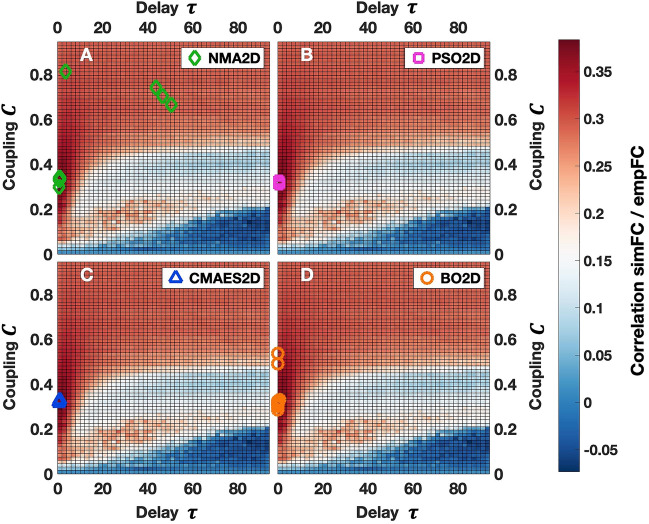
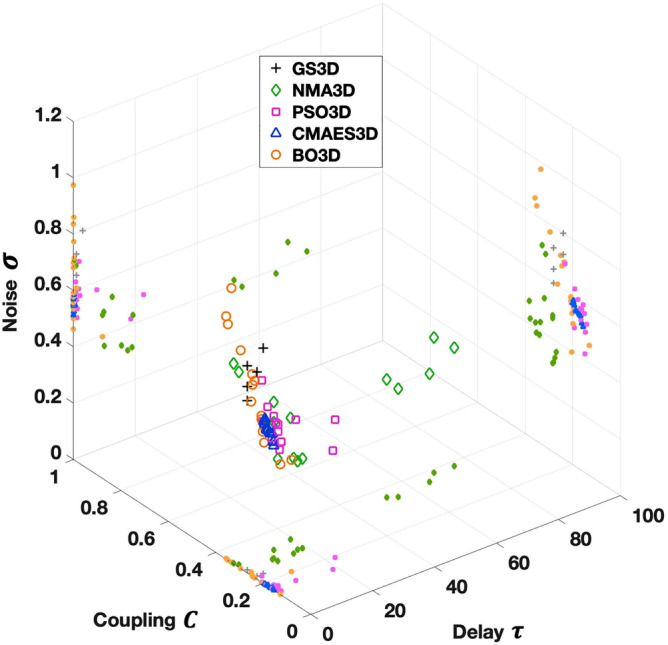
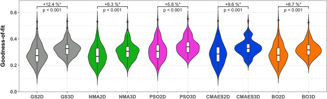
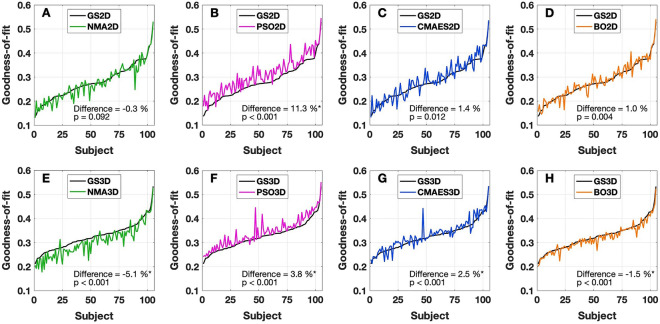
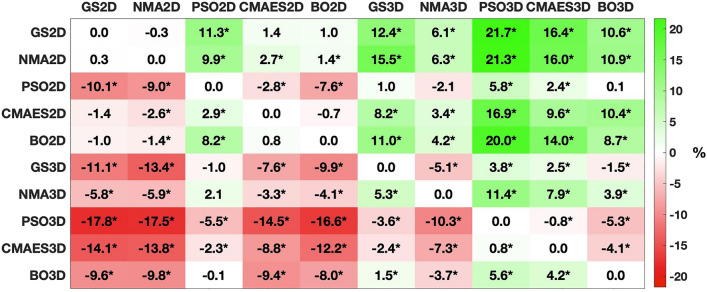
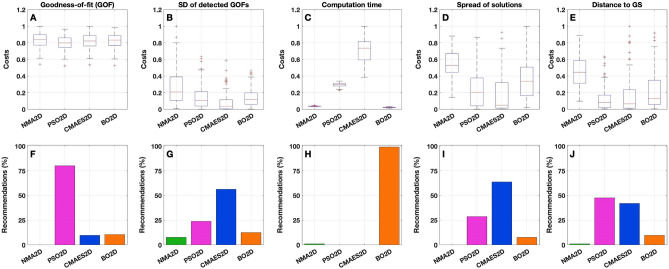
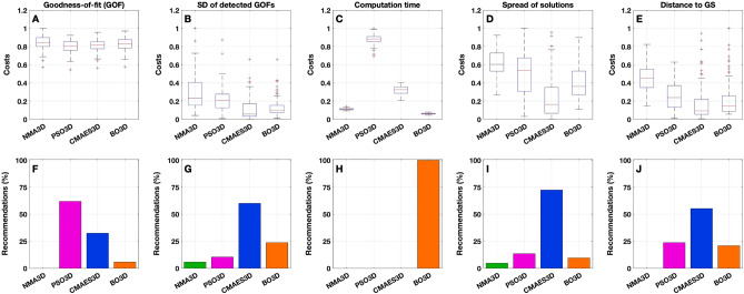
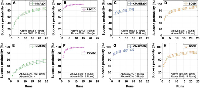
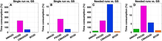
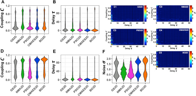
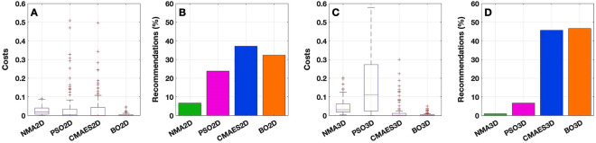
Simulating the resting-state brain dynamics via mathematical whole-brain models requires an optimal selection of parameters, which determine the model's capability to replicate empirical data. Since the parameter optimization via a grid search (GS) becomes unfeasible for high-dimensional models, we evaluate several alternative approaches to maximize the correspondence between simulated and empirical functional connectivity. A dense GS serves as a benchmark to assess the performance of four optimization schemes: Nelder-Mead Algorithm (NMA), Particle Swarm Optimization (PSO), Covariance Matrix Adaptation Evolution Strategy (CMAES) and Bayesian Optimization (BO). To compare them, we employ an ensemble of coupled phase oscillators built upon individual empirical structural connectivity of 105 healthy subjects. We determine optimal model parameters from two- and three-dimensional parameter spaces and show that the overall fitting quality of the tested methods can compete with the GS. There are, however, marked differences in the required computational resources and stability properties, which we also investigate before proposing CMAES and BO as efficient alternatives to a high-dimensional GS. For the three-dimensional case, these methods generated similar results as the GS, but within less than 6% of the computation time. Our results contribute to an efficient validation of models for personalized simulations of brain dynamics.

Figure 1

Examples of the algorithms’ solutions in the 2Dim parameter space. All plots illustrate the outcome for the same subject. As indicated in the legends, the results of the 2Dim parameter optimizations via NMA (NMA2D), PSO (PSO2D), CMAES (CMAES2D) and BO (BO2D) are visualized by colored symbols (diamonds, squares, triangles and circles, respectively). For each method, 15 optimal parameter points obtained from 15 algorithm executions with random initial conditions are indicated. The background fill of the plots illustrates the shape of the parameter space as discovered by the grid search, see also Fig. S1. It shows the similarity (Pearson correlation) between simulated and empirical FC on a color scale reaching from dark blue (low similarity) to dark red (high similarity). The figure was created with MATLAB R2018a (www.mathworks.com).

Figure 2

Exemplary parameter optimization in the 3Dim case. The outcomes (optimal parameter points) for all tested methods are combined in one plot. Besides the solutions in the 3Dim parameter space (larger markers), projections to 2Dim plains are presented (smaller markers). For the grid search in 3Dim (GS3D), five parameter points are considered (black crosses). In terms of the model similarity to empirical data, these points represent the five best solutions out of all values calculated on the parameter grid. As indicated in the legend, the results of the 3Dim parameter optimizations via NMA (NMA3D), PSO (PSO3D), CMAES (CMAES3D) and BO (BO3D) are visualized by colored diamonds, squares, triangles and circles, respectively. For each algorithm, 15 markers are shown (plus projections) which indicate the solutions of 15 runs executed at random initial conditions. The figure was created with MATLAB R2018a (www.mathworks.com).

Figure 3

Distributions of the goodness-of-fit values for all tested approaches and dimensionalities. The considered methods and the respective parameter space’s dimension are indicated on the horizontal axis (GS2D, NMA2D, PSO2D, CMAES2D, BO2D in 2Dim and GS3D, NMA3D, PSO3D, CMAES3D, BO3D in 3Dim) along with the detected goodness-of-fit values on the vertical axis. Violins show the distributions of the highest model fit detected for all subjects. The medians (across subjects) of the relative increase between the results in 2Dim and 3Dim are indicated in the plots together with p-values of the Wilcoxon signed-rank test. Statistically significant differences are marked with an asterisk (the significance level of 5%, p < 0.05, has been Bonferroni-corrected for multiple comparisons).

Figure 4

Goodness-of-fit values for individual subjects and optimization approaches. As indicated in the legends, colored curves illustrate the outcome (subject-dependent goodness-of-fit) for each method in the (A–D) 2Dim (NMA2D, PSO2D, CMAES2D, BO2D) and (E–H) 3Dim (NMA3D, PSO3D, CMAES3D, BO3D) cases. The subjects are sorted in ascending order, based on the maximal fitting values detected by the grid search (black curves) in 2Dim and 3Dim (GS2D and GS3D, respectively). The medians (across subjects) of the relative differences between the results of the optimization algorithms and the grid search are indicated in the plots together with p-values of the Wilcoxon signed-rank test. Statistically significant differences are marked with an asterisk (the significance level of 5%, p < 0.05, has been Bonferroni-corrected for multiple comparisons). The figure was created with MATLAB R2018a (www.mathworks.com).

Figure 5

Comparison of the considered methods with regard to the detected goodness-of-fit values across all subjects. For every optimization technique and subject, the highest goodness-of-fit value is considered. The medians of the relative differences between any two methods are indicated in the cells which are highlighted in color. To this end, the goodness-of-fit values of the approaches listed on the vertical axis (lines) are subtracted from those of the methods indicated on the horizontal axis (columns). Results that proved statistically significant in the Wilcoxon signed-rank test are marked with an asterisk (the significance level of 5%, p < 0.05, has been Bonferroni-corrected for multiple comparisons). The figure was created with MATLAB R2018a (www.mathworks.com).

Figure 6

Components of the cost function $\mathrm{\Psi }$_cost for the 2Dim case. (A–E) Boxplots illustrate the distributions of the values of the components indicated in the titles (see text for details). All values were normalized by the respective maxima (given as one quantity over all algorithms for a given component). The individual cost values are shown on the vertical axes while the corresponding algorithms (NMA2D, PSO2D, CMAES2D and BO2D) are indicated on the horizontal axes. (F–J) For each cost component, histograms show the relative number of recommendations obtained by a given optimization algorithm across all subjects. This quantity was calculated by counting the number of subjects for which the respective algorithm is considered recommendable, i.e. where it provides the lowest costs among all four investigated methods. The absolute value was then divided by the total cohort size of 105 subjects. As before, the methods are listed on the horizontal axes. On the vertical axes, it is indicated for which fraction of subjects a particular method is recommended. The figure was created with MATLAB R2018a (www.mathworks.com).

Figure 7

Components of the cost function $\mathrm{\Psi }$_cost for the 3Dim case. As in Fig. 6, (A–E) boxplots illustrate the distributions of the values (normalized by the respective maxima) of the components indicated in the titles, and (F–J) histograms show the relative number of recommendations obtained by a given optimization algorithm (NMA3D, PSO3D, CMAES3D and BO3D) for each cost component. The figure was created with MATLAB R2018a (www.mathworks.com).

Figure 8

Numbers of algorithm executions and corresponding probabilities to obtain a goodness-of-fit not smaller than 95% of that from the grid search in the 2Dim (A–D) and 3Dim (E–H) cases. The probabilities were evaluated by randomly selecting $R\in \{1,\dots ,R_{max}\}$ goodness-of-fit values from the R_max algorithm executions available for every subject (R_max = 15 for PSO and CMAES, R_max = 24 for NMA and BO). A success was noted when at least one of the selected values was above or equal to the threshold. For every choice of R (i.e. the number of performed runs indicated on the horizontal axes), this procedure was repeated 500 times. The results were then averaged across all subjects in order to obtain the mean success probabilities indicated on the vertical axes. For the optimization methods presented in the legends (same notations as before), the plots illustrate the mentioned success probabilities together with the respective standard error (error bars). Additionally, it is indicated after how many runs success probabilities of 50% and 80% could be surpassed. The figure was created with MATLAB R2018a (www.mathworks.com).

Figure 9

Computation time necessary for the execution of the optimization algorithms in relation to that used for the grid search (GS). (A, B) Ratios between the computation time of a single run of the optimization algorithms and the grid search averaged over all algorithm executions and subjects. The individual ratios are (A) 2Dim case: NMA2D 1.8%, PSO2D 231.0%, CMAES2D 55.6% and BO2D 1.9%; (B) 3Dim case: NMA3D 0.1%, PSO3D 7.7%, CMAES3D 1.9% and BO3D 0.1%. (C, D) Relative computation time necessary for reaching 80% of the success probability (see Fig. 8) compared to the time invested for the grid search. The values are obtained by multiplying those from the plots A and B by the respective numbers of needed runs provided in Fig. 8. For NMA3D, where a success probability of 80% could not be reached, 24 runs are considered necessary. The algorithms are indicated on the horizontal axes along with the percental values of time consumption on the vertical axes for the 2Dim (A, C) and 3Dim (B, D) cases. The figure was created with MATLAB R2018a (www.mathworks.com).

Figure 10

Distributions of the optimal model parameters detected by the considered techniques across all subjects. For each approach and subject, the five best solutions featuring the highest goodness-of-fit values are considered to estimate the distribution. They were selected from all similarity values computed on the 2Dim or 3Dim parameter grids (for the grid search GS2D or GS3D) and from all goodness-of-fit values obtained by 15 independent runs of the optimization algorithms (NMA2D, PSO2D, CMAES2D, BO2D in 2Dim and NMA3D, PSO3D, CMAES3D, BO3D in 3Dim). In the violin plots of one-parameter distributions for the 2Dim (A, B) and 3Dim (D–F) cases, the methods are indicated on the horizontal axes along with the optimized parameter values on the vertical axes. The plots (C1–C5) show the distributions of the optimal model parameters in the 2Dim space, where the relative frequency of the optimal parameter values is depicted by color and the respective methods are indicated in the plots. The figure was created with MATLAB R2018a (www.mathworks.com).

Figure 11

Cost function values and recommendations pertaining to the optimization algorithms for the 2Dim (A, B) and 3Dim (C, D) cases. (A, C) Boxplots illustrate the distribution of costs (normalized by the respective maxima, i.e. one value over all algorithms in the given parameter space). The considered methods are depicted on the horizontal axes together with the values of $\mathrm{\Psi }$_cost on the vertical axes. A few outliers for PSO (> 0.6 in 3Dim) and CMAES (> 0.6 in 2Dim) are not included in the plots. (B, D) Histograms show the relative number of recommendations obtained by a given optimization algorithm (calculated as in Fig. 6). The methods are listed on the horizontal axes. On the vertical axes, it is indicated for which fraction of subjects a particular method is recommended. The figure was created with MATLAB R2018a (www.mathworks.com).

References

1. Biswal B, Yetkin FZ, Haughton VM, Hyde JS. Functional connectivity in the motor cortex of resting human brain using echo-planar MRI. Magn. Reson. Med. 1995;34:537–541. doi: 10.1002/mrm.1910340409. - DOI - PubMed
1. van den Heuvel, M. P. & Hulshoff Pol, H. E. Exploring the brain network: A review on resting-state fMRI functional connectivity. Eur Neuropsychopharmacol20, 519–534. 10.1016/j.euroneuro.2010.03.008 (2010). - PubMed
1. Snyder AZ, Raichle ME. A brief history of the resting state: the Washington University perspective. Neuroimage. 2012;62:902–910. doi: 10.1016/j.neuroimage.2012.01.044. - DOI - PMC - PubMed
1. Cole MW, Bassett DS, Power JD, Braver TS, Petersen SE. Intrinsic and task-evoked network architectures of the human brain. Neuron. 2014;83:238–251. doi: 10.1016/j.neuron.2014.05.014. - DOI - PMC - PubMed
1. Bolt T, Nomi JS, Rubinov M, Uddin LQ. Correspondence between evoked and intrinsic functional brain network configurations. Hum. Brain Mapp. 2017;38:1992–2007. doi: 10.1002/hbm.23500. - DOI - PMC - PubMed
Publication types