Systematic reconstruction of cellular trajectories across mouse embryogenesis

Abstract

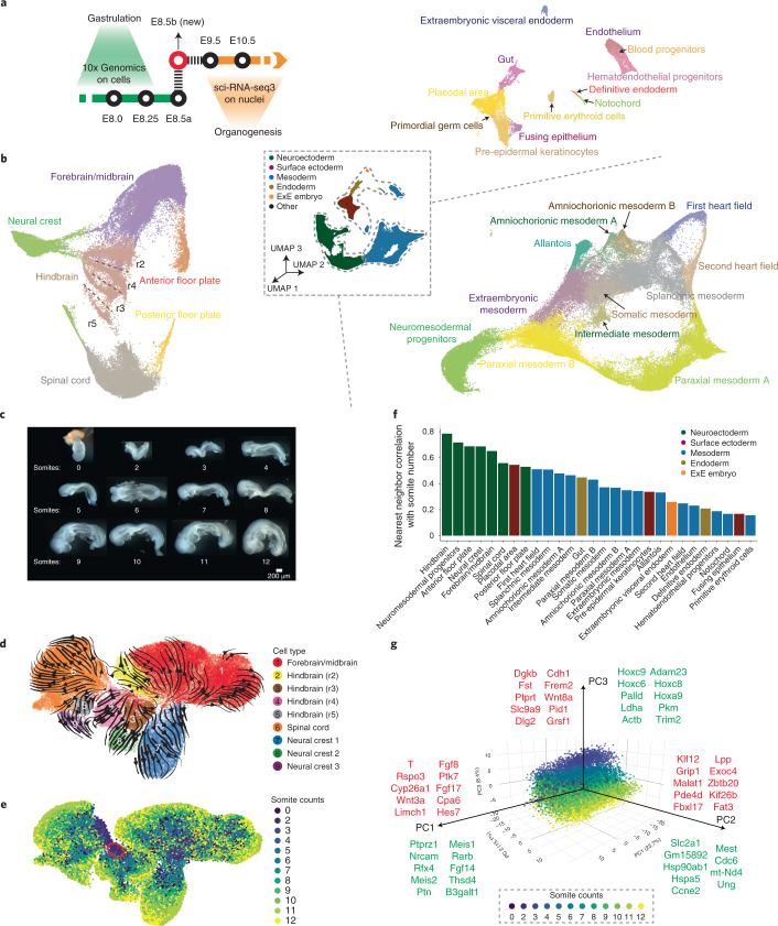
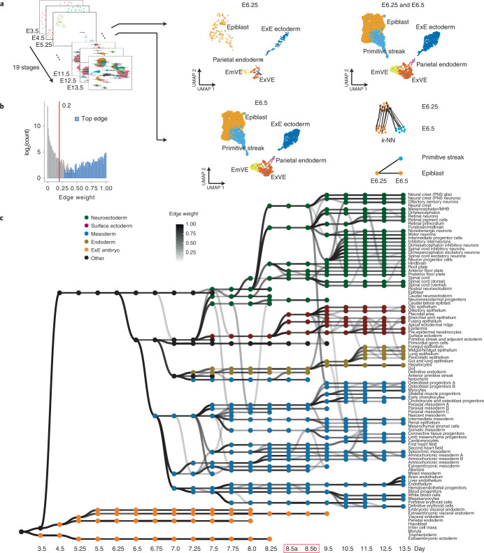
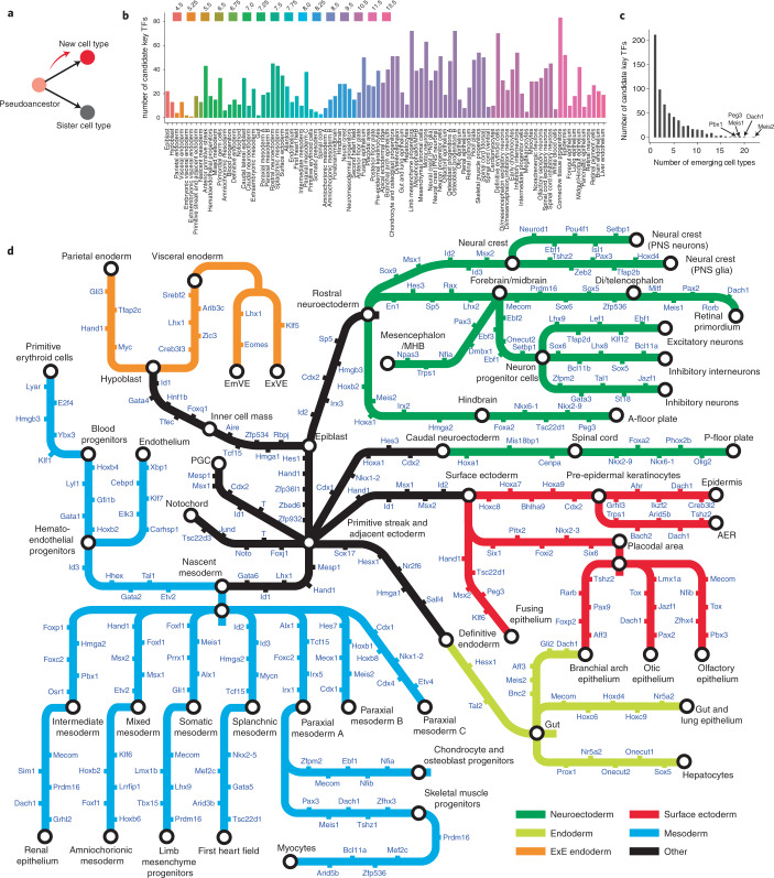
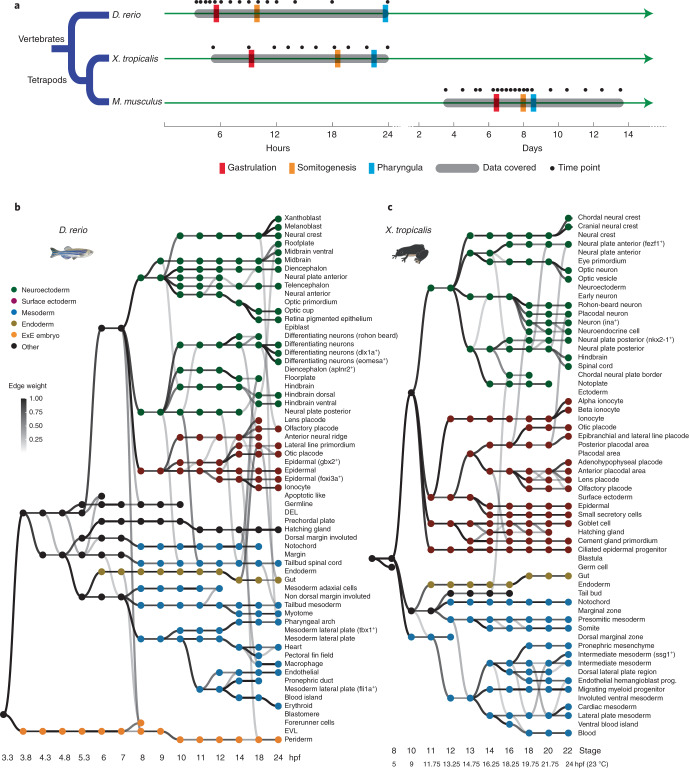
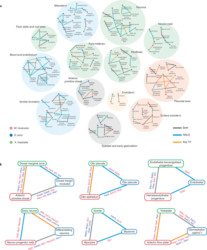
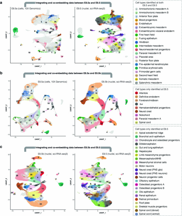
Mammalian embryogenesis is characterized by rapid cellular proliferation and diversification. Within a few weeks, a single-cell zygote gives rise to millions of cells expressing a panoply of molecular programs. Although intensively studied, a comprehensive delineation of the major cellular trajectories that comprise mammalian development in vivo remains elusive. Here, we set out to integrate several single-cell RNA-sequencing (scRNA-seq) datasets that collectively span mouse gastrulation and organogenesis, supplemented with new profiling of ~150,000 nuclei from approximately embryonic day 8.5 (E8.5) embryos staged in one-somite increments. Overall, we define cell states at each of 19 successive stages spanning E3.5 to E13.5 and heuristically connect them to their pseudoancestors and pseudodescendants. Although constructed through automated procedures, the resulting directed acyclic graph (TOME (trajectories of mammalian embryogenesis)) is largely consistent with our contemporary understanding of mammalian development. We leverage TOME to systematically nominate transcription factors (TFs) as candidate regulators of each cell type's specification, as well as 'cell-type homologs' across vertebrate evolution.

Fig. 1. Intensive scRNA-seq of somite-resolved E8.5 mouse embryos.

a, A new scRNA-seq dataset was generated from nuclei derived from individual E8.5 mouse embryos via an optimized sci-RNA-seq3 protocol to bridge existing data generated on E8.5 cells via 10x Genomics and E9.5 nuclei via sci-RNA-seq3 (ref. ). b, 3D UMAP visualizations of the new E8.5 dataset (E8.5b). All nuclei colored by germ layer are shown in the center, along with separate embeddings of neuroectoderm (left), nonhematopoietic mesoderm (bottom right) and endoderm, extraembryonic and hematopoietic cell types (top right). c, Twelve mouse embryos, including a single primitive-streak-stage embryo and 11 embryos staged in 1-somite increments from 2 to 12 somites, were collected and their nuclei subjected to optimized sci-RNA-seq3. d, Re-embedded two-dimensional (2D) UMAP of cells annotated as forebrain, midbrain, hindbrain, spinal cord and neural crest. Arrows correspond to RNA velocity trends. e, The same UMAP as in d, colored by somite counts. The subset of cells from rhombomere 4 that appear to emerge the earliest are highlighted in red circles (Hoxa1⁺ and Hoxb1⁺)^,. f, For each cell type with >100 profiled cells, we calculated the Pearson correlation coefficient between the somite number of each cell of that type and the average somite number of its five nearest neighbors in the global 3D UMAP embedding. Colors indicate germ layers. g, 3D visualization of the top three PCs of gene expression variation in NMPs, calculated on the basis of the 2,500 most highly variable genes. Cells are colored by the somite count of the originating embryo. Genes most strongly correlated (Pearson), either positively (red) or negatively (green), with each PC are listed. ExE, extraembryonic; r2–r5: rhombomeres 2–5.

Fig. 2. Systematic reconstruction of the cellular trajectories of mouse embryogenesis.

a, Overview of approach. Cells from each pair of adjacent stages were projected into the same embedding space. UMAP visualizations of coembedded cells from E6.25 and E6.5 are shown separately (middle column) or together (top right). A k-NN heuristic was applied to infer one or several pseudoancestors for each of the cell states observed at the later time point (bottom right). b, Histogram of all calculated edge weights. The y axis is on a log₂ scale. Edges with weights above 0.2 (red line) were retained. Top edges are those with the highest weight amongst all potential antecedents of each cell state. c, Directed acyclic graph showing inferred relationships between cell states across early mouse development. Each row corresponds to one of 94 cell-type annotations, columns to developmental stages spanning E3.5 to E13.5, nodes to cell states and node colors to germ layers. All edges with weights above 0.2 are shown in grayscale. Of note, placental tissues were not actively retained during the isolation of embryos from later time points. E8.5a and E8.5b were essentially treated as two distinct time points, because they are bridging datasets that are substantially different from a technical perspective (Fig. 1a and Extended Data Fig. 2). Di, diencephalon; EmVE, embryonic visceral endoderm; ExE, extraembryonic; ExVE, extraembryonic visceral endoderm; MHB, midbrain–hindbrain boundary; PNS, peripheral nervous system.

Fig. 3. RNA velocity and spatially correlated coembeddings clarify relationships between cell types during neuronal differentiation, hematopoiesis and neural tube development.

a, RNA velocity was estimated on the basis of the proportion of reads mapping to exonic versus intronic portions of genes using scVelo (ref. ). Cells corresponding to motor neurons, noradrenergic neurons, di/mesencephalon inhibitory neurons, spinal cord inhibitory neurons, di/mesencephalon excitatory neurons, spinal cord excitatory neurons, inhibitory interneurons, intermediate progenitor cells and neuron progenitor cells from E9.5 to E13.5 were included in this analysis, after downsampling each cell state to 5,000 cells. UMAP visualization of coembedded cells and cell-state transition trends (arrows) are shown. Smaller panels show the same UMAP visualization but with coloring of cells from individual time points. b, Same as a, but for cells corresponding to blood progenitors, white blood cells, megakaryocytes, definitive erythroid cells and primitive erythroid cells from E8.5b to E13.5. c, UMAP visualization of coembedded cells from neural tube derivatives from E8.5b and E9.5 data after batch correction. The same UMAP is shown twice for both, with colors highlighting cells and corresponding annotations from either E8.5b (top) or E9.5 (bottom).

Fig. 4. Inference of the approximate spatial locations of cell states during mouse gastrulation.

a, Inference of cell-type contributors to each spatial territory of the gastrulating mouse embryo based on the application of CIBERSORTx to GEO-seq data^,. GEO-seq yields bulk RNA-sequencing data from small numbers of cells dissected from precise anatomic regions of the gastrulating embryo. We then estimated the proportional contribution of each cell state to each GEO-seq sample using CIBERSORTx (ref. ). b, Corn plots showing the spatial pattern of inferred contributions of various ectodermal cell types at E7.5. c, Corn plots showing the spatial pattern of inferred contributions of various mesodermal cell types at E7.5. d, Corn plots showing the spatial pattern of inferred contributions of various endodermal cell types at E7.5, as well as notochord. In each corn plot, each circle or diamond refers to a GEO-seq sample and its weighted color to the estimated cell-type composition. Corn plot nomenclature from Peng et al.. A, anterior; P, posterior; L, left lateral; R, right lateral; L1, anterior left lateral; R1, anterior right lateral; L2, posterior left lateral; R2, posterior right lateral; Epi1 and Epi2, divided epiblast; M, whole mesoderm; MA, anterior mesoderm; MP, posterior mesoderm; En1 and En2, divided endoderm; EA, anterior endoderm; EP, posterior endoderm.

Fig. 5. Systematic nomination of candidate key TFs for cell-type specification.

a, We heuristically defined candidate key TFs as those that are expressed in the pseudoancestral cell state, are significantly upregulated in the newly emerged cell type and are not significantly upregulated at any sister edges. b, Histogram of the number of candidate key TFs for each cell type at the time point of its first emergence. c, The histogram of the number of cell types in which each TF was nominated as a candidate key TF. d, Diagram illustrating selected cellular trajectories from TOME, decorated with the top five scoring candidate key TFs for each edge. AER, apical ectodermal ridge. Style inspired by Morris et al..

Fig. 6. Reconstruction of the cellular trajectories of zebrafish and frog embryogenesis.

a, Comparative developmental timelines for mouse, zebrafish and frog, spread over two time scales, and approximate (as temperature dependent, particularly for frog). Gastrulation and somitogenesis refer to the timing of onset of these processes. Pharyngula refers to the timing of onset of PA formation. Black dots refer to time points sampled across seven studies. Gray rounded rectangles indicate developmental windows covered by cellular trajectory reconstructions. b, Directed acyclic graph showing inferred relationships between cell states across early zebrafish development. Each row corresponds to one of 63 cell-type annotations and columns to developmental stages spanning hours postfertilization 3.3 (hpf3.3) to hpf24. Nodes denote cell states, and node colors denote germ layers. All edge weights greater than 0.2 are shown in grayscale. c, Directed acyclic graph showing inferred relationships between cell states across early frog development. Each row corresponds to one of 60 cell-type annotations, columns to developmental stages spanning S8 (hpf5, 23 °C) to S22 (hpf24, 23 °C), nodes to cell states and node colors to germ layers. All edge weights greater than 0.2 are shown in grayscale. DEL, deep cell layer; EVL, enveloping layer.

Fig. 7. The union of candidate cell-type homologs, identified among three species (mouse, zebrafish and frog) by two strategies.

a, Candidate cell-type homologs were identified either by comparison of transcriptomes via nonnegative least-squares regression or by examining overlap between upregulated candidate key TFs (key TF). Nominated pairings were manually reviewed, and a subset retained based on biological plausibility. Colors of nodes indicate the species of a given cell type, and colors of edges indicate which approach(es) identifies the pairing. Sets of connected candidate cell-type homologs are further grouped by germ layer or developmental system. b, Selected examples of ‘three-way’ pairwise cell-type homology from different germ layers in the above network. Upregulated candidate key TFs shared by each pair of species are listed, with the subset shared by all three species in red font. Of note, key TFs shared by mouse (mm) versus zebrafish (zf) and mm versus frog (xp) are shown by mouse gene symbols, whereas key TFs shared by zf versus xp are shown by zebrafish gene symbols. NNLS, nonnegative least squares.

Extended Data Fig. 1. Integration of datasets generated by different groups using different scRNA-seq technologies.

a, As illustrated by a UMAP of coembedded E6.5 cells, batch effects are observed between three studies, as well as different embryos from the same study. The same UMAP is shown several times on the bottom of the panel, with colors highlighting cells from different studies or samples. b, UMAP of the same cells as in panel a with batch correction prior to integration. The same UMAP is shown several times on the bottom of the panel, with colors highlighting cells from different studies or samples. In addition, the same UMAP is shown on the upper right, but colored by cell-type annotation. c, UMAP visualization of co-embedding of data from E8.5a (cells) generated on the 10x Genomics platform and E9.5 (nuclei) generated using sci-RNA-seq3, before batch correction. The same UMAP is shown twice for both, with colors highlighting cells from either E8.5a (left) or E9.5 (right). E9.5 profiles were based on deeper sequencing of the same libraries reported in Cao et al.. d, UMAP of the same cells as in panel c but with batch correction prior to integration. Left and right as in panel c. ExE: extraembryonic. EmVE: embryonic visceral endoderm. ExVE: extraembryonic visceral endoderm.

Extended Data Fig. 2. Integrating and coembedding cells from E8.5a, E8.5b and E9.5.

For panels a and c, E9.5 profiles were based on deeper sequencing of the same libraries reported in Cao et al.. a, UMAP visualization of coembedded cells at E8.5a generated on the 10x Genomics platform and nuclei at E9.5 generated using sci-RNA-seq3 after batch correction. The same UMAP is shown twice for both, with colors highlighting cells/nuclei from either E8.5a (left) or E9.5 (right). b, UMAP visualization of coembedded cells at E8.5a generated on the 10x Genomics platform and nuclei at E8.5b generated using sci-RNA-seq3 after batch correction. The same UMAP is shown twice for both, with colors highlighting cells/nuclei from either E8.5a (left) or E8.5b (right). c, UMAP visualization coembedded nuclei at E8.5b and nuclei at E9.5, both generated with sci-RNA-seq3, after batch correction. The same UMAP is shown twice for both, with colors highlighting nuclei from either E8.5b (left) or E9.5 (right).

Extended Data Fig. 3. Resolution of hindbrain segmentation in newly created E8.5 dataset.

a, Subview of global 3D UMAP visualization highlighting subsets of cells annotated as rhombomeres 1 - 6 (r1 - 6) in E8.5 data generated with optimized sci-RNA-seq3 protocol. b, Re-embedded 2D UMAP of cells annotated as forebrain, midbrain, presumptive cerebellum, r1–r6, spinal cord and neural crest, although neural crest cells are excluded from visualization. c, The same UMAP as in panel b, colored by gene expression of marker genes used for annotation of anatomical regions. Telencephalon: Otx2+, Fgf8 + ; Diencephalon: Otx2+, En1-, En2-; Midbrain: Otx2+, En1+, En2+, Fgf8-; MHB (midbrain–hindbrain boundary): boundary of Fgf8 and Wnt1; Presumptive cerebellum: Fgf8+, En1+, En2+, Wnt1-, Gbx2 + ; r1: a ‘wedge’ between cerebellum and r2, Fgf8-, Hoxa2-; r2: Fst+, Hoxa2+, Hoxb2-; r3: Egr2+, Hoxb2+, Hoxa3-, Hoxb3-; r4: Fst+, Hoxa1+, Hoxb1+, Hoxa3-, Hoxb3-; r5: Egr2+, Hoxa3+, Hoxb3+, Mafb + ; r6: Mafb+, Egr2-, Hoxb4-^,,–. The subset of cells from r4 which appear to emerge earlier than the other rhombomeres cells are highlighted by red circles in the third row (Hoxa1+, Hoxb1+)^,. d, The same UMAP as in panel b, colored by gene expression of marker genes for the dorsal-ventral axis (Wnt1 is a dorsal marker; Nkx6-1, Foxa2 and Nkx2-2 are ventral markers)^,. The same genes are highlighted in the 3D subview of panel a are shown below. Gene expression values shown in panel c-d were calculated by normalizing the UMI counts by the estimated size factors followed by log10-transformation.

Extended Data Fig. 4. Decoding of transcriptional heterogeneity within NMPs.

a, Subview of global 3D UMAP visualization highlighting spinal cord (blue), neuromesodermal progenitors (red), and paraxial mesoderm B (green). b, The same 3D UMAP as panel a but zooming in to highlight NMP cells, colored according to expression levels of markers of mesodermal (Tbx6, T) or neuroectodermal (Sox2) state^,. Gene expression values were calculated by normalizing the UMI counts by the estimated size factors followed by log10-transformation. c, Embeddings of NMP cells (n = 14,869 cells) in PCA space with visualization of top three PCs, calculated on the basis of the 2,500 most highly variable genes, in 2D. Cells are colored by the somite count of the originating embryo. d, Correlations between top three PCs (rows 1-3) and the normalized expression of selected genes (Tbx, T, Sox2; columns 1-3), cell cycle indices (columns 4-5) or somite counts (column 6) (n = 14,869 cells). Red boxes highlight the strongest absolute correlation in each row. Coefficients and unadjusted p-values were calculated by two-sided Pearson correlation and are shown above the plots. Gene expression values were calculated from original UMI counts normalized to total UMIs per cell, followed by natural-log transformation. Cell cycle indices were estimated using the CellCycleScoring function of Seurat/v3 (S.Score and G2M.Score). e, The 114 genes most strongly correlated with PC3 (which appears to correlate to somite counts) were identified using two-sided Pearson correlation (out of the 5,000 most variable genes; FDR < 0.05 and absolute coefficients > 0.2; Supplementary Table 3). The sklearn.svm.LinearSVR function in scikit-learn/1.0 was applied to assess whether the somite counts of the originating embryos of NMP cells could be predicted from their transcriptional profiles. The distributions of true (x-axis) vs. predicted (y-axis) somite counts for NMP cells are shown, without (top) or with (bottom) permutation of somite count labels (n = 14,869 cells). Coefficients and unadjusted p-values were calculated by two-sided Pearson correlation and are shown above the plots. In the boxplots shown in panel d and e, the center lines show the medians; the box limits indicate the 25th and 75th percentiles; the whiskers extend to the 5th and 95th percentiles; the outliers are represented by the dots.

Extended Data Fig. 5. Integration of datasets spanning E3.5 to E13.5 of mouse development.

a, The number of cells per stage obtained from three previous studies^,,, new E8.5 data obtained via optimized sci-RNA-seq3, and deeper sequencing of Cao et al.. b, The number of cells per embryo corresponding to specific somite counts from new E8.5 data. c, Box plot of log2(UMI counts) per cell across the stages and studies (n = 1,658,968 cells).The center lines show the medians; the box limits indicate the 25th and 75th percentiles; the whiskers extend to the 5th and 95th percentiles; the outliers are represented by the dots. d, The same strategy of creating the edges between adjacent time points was performed after randomly shuffling the cell-state annotations for cells within each time point, followed by repeating this process 1,000 times, resulting in a null distribution of edge weights. After permutation, less than 1% of potential edges are assigned weights greater than 0.2 (red line). e, To quantify the quality of the integration between adjacent time points, we focused on cells at the later time point assigned to annotations that were also present at the earlier time point. We then calculated the fraction of these cells’ ancestral k-nearest neighbors (in the global 3D UMAP co-embedding) that were assigned the identical annotation. The mean proportion for different values of k are reported in the histogram. Of note, the lower value of this metric for E8.5a-E9.5 (red label) than E8.5a-E8.5b or E8.5b-E9.5 provides quantitative support for our claim that the new E8.5b data improved integration across the E8.5 to E9.5 (Extended Data Fig. 2).

Extended Data Fig. 6. TOME edges nominated by k-NN versus RNA velocity-based heuristics are largely concordant.

a, Histogram of all potential edge weights calculated by RNA velocity. The y-axis is on a log2 scale. Edges with weights above 0.2 (red line) were retained. b, After calculating the transition probability for individual cells between adjacent time points using scVelo, the same strategy of creating the edges was performed after randomly shuffling the cell-state annotations for cells within each time point, followed by repeating this process 1,000 times, resulting in a null distribution of edge weights. After permutation, less than 1% of potential edges are assigned weights greater than 0.2 (red line). c, Ignoring edges prior to E6.5 as well as between E8.5a and E8.5b (see text), out of 15,261 potential edges, there were 123 edges nominated by the k-NN strategy only (weight > 0.2), and 75 edges nominated by the RNA velocity strategy only (weight > 0.2), and 392 nominated by both strategies. d, Directed acyclic graph showing inferred relationships between cell states across early mouse development. Layout identical to Fig. 2c. Each row corresponds to one of 94 cell-type annotations, columns to developmental stages spanning E3.5 to E13.5, nodes to cell states, and node colors to germ layers. Edges nominated with weights above 0.2 by RNA velocity only are shown in red, by k-NN in blue, and by both strategies in purple. ExE: extraembryonic. PNS: peripheral nervous system. MHB: midbrain–hindbrain boundary. Di: diencephalon.

Extended Data Fig. 7. Estimated cell-type proportions for different regions of the gastrulating mouse embryo, arranged by inferred cell-type relationships over time.

a, The inferred cell–state proportions of each GEO-seq territory are robust to downsampling. For time point which GEO-seq data was available (E5.5, E6.0, E6.5, E7.0, and E7.5), we estimated a gene expression signature for each cell state from scRNA-seq data, either by using all the cells or by downsampling to a maximum of 50 cells per state, and then repeated the inference of cell-type contributors to each spatial territory of the gastrulating mouse embryo based on the application of CIBERSORTx to GEO-seq data^,. The Pearson correlation of resulting estimated cell–state proportions for each GEO-seq territory with downsampling (y-axes) or without downsampling (x-axes) are shown. Of note, we did not use downsampling in the results shown in Fig. 4b, As described in Fig. 4a, inference of cell-type contributor(s) to each spatial territory of the gastrulating mouse embryo based on the application of CIBERSORTx to GEO-seq data^,. As scRNA-seq data from E6.0 was unavailable, we used data from E6.25 instead. Black edges correspond to edges between cell states over time estimated by TOME (only edges with the largest weights are shown). In each corn plot, each circle or diamond refers to a GEO-seq sample, and its weighted color to the estimated cell-type composition. Corn plot nomenclature from Peng et al.. A, anterior; P, posterior; L, left lateral; R, right lateral; L1, anterior left lateral; R1, anterior right lateral; L2, posterior left lateral; R2, posterior right lateral; Epi1 and Epi2, divided epiblast; M, whole mesoderm; MA, anterior mesoderm; MP, posterior mesoderm; En1 and En2, divided endoderm; EA, anterior endoderm; EP, posterior endoderm.

Extended Data Fig. 8. Correlation between key TF expression and up- or downregulation of putative targets of regulation.

a, UMAP visualization of coembedded cells from cell states including anterior primitive streak, definitive endoderm, gut, and notochord (mouse E7.25 → E7.5) colored by cell type (left), Rfx3 gene expression (middle) or RFX3 motif score (right), respectively. The RFX3 motif score for each cell was calculated by averaging the gene expression of 135 key genes for notochord emergence bearing this motif in their core promoters, and then subtracting the mean expression of a reference set of randomly sampled genes, using the score_genes function of Scanpy. b, Positional bias of RFX3 binding motif along the core promoters of key genes for notochord emergence (right panel), an expanded region for key genes for notochord emergence (left top panel), or an expanded region for background (left bottom panel). The y-axes indicate the % of key genes or background genes with the RFX3 motif with 10 bp bins. c, The motif logo of the top de novo motif for notochord emergence and its two best alignments in the known motif database. d, UMAP visualization of coembedded cells from cell states including primitive streak and nascent mesoderm (mouse E6.5 → E7.25) colored by cell types (left), Snai1 gene expression (middle) or SNAIL1 motif score (right), respectively. The SNAIL1 motif score was calculated as in panel a, based on 21 key genes for nascent mesoderm emergence bearing this motif in their core promoters. e, Positional bias of SNAI1 binding motif along the core promoters of key genes for nascent mesoderm emergence (right panel), an expanded region for key genes for nascent mesoderm emergence (left top panel), or an expanded region for background (left bottom panel). The y-axes indicate the % of key genes or background genes with the SNAIL1 motif with 10 bp bins. f, The known motif logo of SNAIL1.

Extended Data Fig. 9. Coembedding of 825 cell states from three species by integrating their transcriptional features.

For cell states spanning multiple time points, cells from each time point were treated separately for the purposes of this analysis. To create a transcriptional feature corresponding to each cell state (that is a pseudocell), we first averaged cell-state-specific UMI counts, normalized by the total count, multiplied by 100,000 and natural-log-transformed after adding a pseudocount. We then divided all resulting 825 pseudo-cells from the three species into four groups: the mouse single-cell group (n = 151), the mouse single-nucleus group (n = 277), the zebrafish group (n = 205), and the frog group (n = 192), and performed the anchor-based batch correction. UMAP visualization shows coembedded pseudo-cells from the mouse (red), the zebrafish (blue), and the frog (green). Each circle corresponds to a pseudocell, and the numbers correspond to the cell–state labels shown below. The grey dotted curves (manually added) highlight 15 major groups, each including representatives from all three species. Cell states from the extraembryonic lineages (inner cell mass, hypoblast, parietal endoderm, extraembryonic ectoderm, visceral endoderm, embryonic visceral endoderm, and extraembryonic visceral endoderm for the mouse; blastomere, EVL, periderm, forerunner cells for the zebrafish) were excluded from this analysis. For E6.5 of mice, we only used cells from a single study. PNS: peripheral nervous system. MHB: midbrain–hindbrain boundary. Di: diencephalon. DEL: deep cell layer. EVL: enveloping layer.

Extended Data Fig. 10. Correlated cell types between species based on nonnegative least-squares regression.

a, Correlated cell types between each pair of species based on nonnegative least-squares (NNLS) regression (Methods). Shown here is a heat map of the normalized β values between 87 cell types from the mouse, 59 cell types from the zebrafish, and 60 cell types from the frog. The order of cell types listed in the heat map is the same as each cellular trajectory plot (Fig. 2c; Fig. 6b,c). PNS: peripheral nervous system. MHB: midbrain–hindbrain boundary. Di: diencephalon. DEL: deep cell layer. b, The log2-scaled number of all possible pairs, highly ranked pairs, and biologically plausible pairs of cell types evaluated by nonnegative least-squared (NNLS) regression. ‘All possible pairs’ refers to all potential cell type pairings considered; ‘highly ranked pairs’ refer to pairings with β > 1e-4 and that ranked highly from the perspective of both species; ‘plausible pairs’ refer to pairings which were retained after manual review for biological plausibility (Supplementary Table 23). Actual numbers are shown above each bar, with y-axis on log2 scale. c, The log2-scaled number of all possible pairs, highly ranked pairs, and biologically plausible pairs of cell types evaluated on the basis of overlapping, orthologous candidate key TFs. ‘All possible pairs’ refers to all potential cell type pairings considered; ‘highly ranked pairs’ refer to pairings with with estimated relative likelihoods more extreme than 99% of permutations; ‘plausible pairs’ refer to pairings which were retained after manual review for biological plausibility (Supplementary Table 24). Actual numbers are shown above each bar, with y-axis on log2 scale.

References

1. Sulston JE, Schierenberg E, White JG, Thomson JN. The embryonic cell lineage of the nematode Caenorhabditis elegans. Dev. Biol. 1983;100:64–119. doi: 10.1016/0012-1606(83)90201-4. - DOI - PubMed
1. Pijuan-Sala B, et al. A single-cell molecular map of mouse gastrulation and early organogenesis. Nature. 2019;566:490–495. doi: 10.1038/s41586-019-0933-9. - DOI - PMC - PubMed
1. Wagner DE, et al. Single-cell mapping of gene expression landscapes and lineage in the zebrafish embryo. Science. 2018;360:981–987. doi: 10.1126/science.aar4362. - DOI - PMC - PubMed
1. Cao J, et al. The single-cell transcriptional landscape of mammalian organogenesis. Nature. 2019;566:496–502. doi: 10.1038/s41586-019-0969-x. - DOI - PMC - PubMed
1. Briggs JA, et al. The dynamics of gene expression in vertebrate embryogenesis at single-cell resolution. Science. 2018;360:eaar 5780. doi: 10.1126/science.aar5780. - DOI - PMC - PubMed
Publication types