. 2022 Mar;603(7903):878-884.
doi: 10.1038/s41586-022-04515-5. Epub 2022 Mar 16.

A multidimensional coding architecture of the vagal interoceptive system

Affiliations

A multidimensional coding architecture of the vagal interoceptive system

Qiancheng Zhao et al. Nature. 2022 Mar.

Abstract

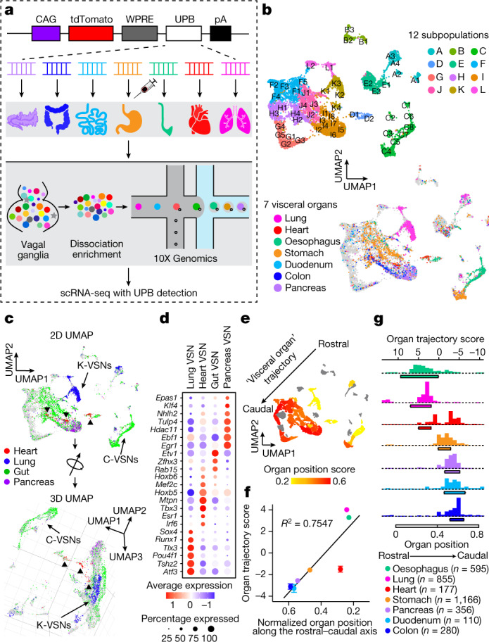
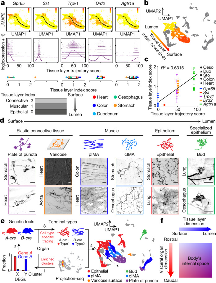
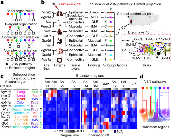
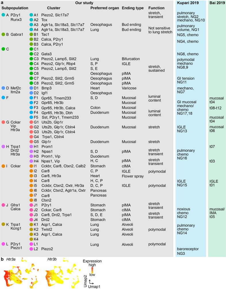
Interoception, the ability to timely and precisely sense changes inside the body, is critical for survival1-4. Vagal sensory neurons (VSNs) form an important body-to-brain connection, navigating visceral organs along the rostral-caudal axis of the body and crossing the surface-lumen axis of organs into appropriate tissue layers5,6. The brain can discriminate numerous body signals through VSNs, but the underlying coding strategy remains poorly understood. Here we show that VSNs code visceral organ, tissue layer and stimulus modality-three key features of an interoceptive signal-in different dimensions. Large-scale single-cell profiling of VSNs from seven major organs in mice using multiplexed projection barcodes reveals a 'visceral organ' dimension composed of differentially expressed gene modules that code organs along the body's rostral-caudal axis. We discover another 'tissue layer' dimension with gene modules that code the locations of VSN endings along the surface-lumen axis of organs. Using calcium-imaging-guided spatial transcriptomics, we show that VSNs are organized into functional units to sense similar stimuli across organs and tissue layers; this constitutes a third 'stimulus modality' dimension. The three independent feature-coding dimensions together specify many parallel VSN pathways in a combinatorial manner and facilitate the complex projection of VSNs in the brainstem. Our study highlights a multidimensional coding architecture of the mammalian vagal interoceptive system for effective signal communication.


Conflict of interest statement

The authors declare no competing interests.

Figures

Fig. 1
Fig. 1. ‘Visceral organ’ coding in VSNs.
a, Schematic illustration of Projection-seq analysis of VSNs innervating the lung, heart, oesophagus, stomach, duodenum, transverse colon and pancreas. Organ illustrations were adapted from BioRender.com. b, UMAP plot from Projection-seq of 14,590 Phox2b+ VSNs (30 mice divided into 4 samples) showing 52 clusters (A1–L2) in 12 VSN subpopulations (A–L) (top) or VSNs expressing UPBs representing 7 visceral organs (colour-coded) (bottom). c, Two-dimensional (2D) (top) and three-dimensional (3D) (bottom) UMAP plots of VSNs innervating different physiological systems. E-VSNs were excluded. The three heart VSN groups (red, arrowheads) are clustered together away from other gut VSNs (green) in the 3D UMAP plot. d, Dot plot showing transcription factors that are differentially expressed in lung, heart, gut and pancreas VSNs. e, UMAP plot of VSN clusters, coloured by target preference (weighted organ position score), showing a ‘visceral organ’ trajectory (arrow) coding visceral organs along the body’s rostral–caudal axis. f, Correlation between the normalized position of the indicated organs along the body’s rostral–caudal axis (mean; n = 4) and the position of VSNs expressing indicated organ UPBs along the ‘visceral organ’ trajectory (organ trajectory score; mean ± s.e.m.; n as indicated). Linear regression R2 = 0.7547. g, Histograms showing the distributions of UPB-labelled VSNs (colour-coded) along the identified ‘visceral organ’ trajectory. The bars underneath indicate normalized organ positions along the body’s rostral–caudal axis (beginning–end; mean ± s.e.m.; n = 4). Source Data
Fig. 2
Fig. 2. A ‘tissue layer’ dimension coding VSN ending locations and structures.
a, UMAP plots of identified DEGs (top) and their expression measures (middle) along a ‘tissue layer’ trajectory. Bottom, DEG+ VSN ending locations, quantified as ‘tissue layer’ index score in corresponding DEGtdT mice (mean; number of mice: Gpr65-oesophagus, 3; Gpr65-stomach, 7; Gpr65-duodenum, 4; Sst-stomach, 5; Trpv1-oesophagus, 3; Trpv1-stomach, 7; Trpv1-duodenum, 4; Trpv1-colon, 4; Trpv1-heart, 10; Drd2-oesophagus, 3; Drd2-stomach, 6; Drd2-duodenum, 3; Drd2-colon, 2; Drd2-heart, 6; Agtr1a-oesophagus, 4; Agtr1a-stomach, 12; Agtr1a-duodenum, 4; Agtr1a-colon, 3; Agtr1a-heart, 6). b, UMAP plot of VSN clusters, coloured by average tissue index determined in Gpr65tdT (F1–F4 clusters; golden), SsttdT (F5 cluster; yellow), Drd2tdT (J2–J4, H2, H4 and I1 clusters; orange), and Agtr1atdT (I2 and I4–6 clusters; orange-red) mice, showing a continuous trajectory coding tissue layers along the organ’s surface–lumen axis. c, Correlation between mean ‘tissue layer’ trajectory score of DEG+ VSNs and their ‘tissue layer’ index score in corresponding DEGtdT mice (mean ± s.e.m.; n as in a). Linear regression R2 = 0.6315. d, VSN ending types characterized in Vglut2tdT mice show stereotypical structures along various tissue layers across multiple visceral organs. Scale bars, 100 μm. e, Projection-seq-guided anterograde tracing (schematic illustration, left) reveals genetic identities of stereotypical VSN ending types illustrated on the UMAP plot (right). VSN clusters forming various VSN ending types followed the ‘tissue layer’ trajectory well (dashed arrow). f, Model for combinatorial coding of the body’s internal space in VSNs using a 2D genetic matrix. Source Data
Fig. 3
Fig. 3. vCatFISH analysis reveals a third ‘stimulus modality’ coding dimension in VSNs.
a, Schematic illustration of vCatFISH analysis. Organ illustrations were adapted from BioRender.com. b, Time-resolved responses (ΔF/F; colour-coded) of 311 single VSNs to the indicated stimuli (lung stretch: oxygen, 600 ml min−1, 20 s; oesophagus and stomach stretch: saline, 100, 300, 600 μl, 30 s; duodenum stretch: saline, 600 μl) in Gpr65tdT-GCaMP6s mice (n = 6) with RNAscope codes (Extended Data Fig. 9c) and annotated subpopulations (A–L). c, VSN subpopulations show stereotypical response patterns across organs (ΔF/F; mean ± s.e.m.; number of VSNs as indicated). Lung stretch responses were aligned at the activation frame (red arrowhead) to reveal response kinetics. Bars represent oesophagus and stomach stretch; black arrowheads represent duodenal stretch (saline, 600 μl). d, VSN endings are uncoupled from response patterns. Left, F-VSNs (Gpr65tdT) and G-VSNs (ViptdT) form indistinguishable mucosal villi endings (ME) in the intestine but respond to different sensory cues (bottom, 5 mice). Middle, pIMAs formed by H/J-VSNs (P2ry1tdT) and C-VSNs (Piezo2tdT) have distinct response kinetics to oesophagus and stomach stretch (bottom, ΔF/F at post-activation frame 15 (f15), mean ± s.e.m., 5 mice, ***P < 0.001, P = 7.4 × 10−7, two-tailed t-test). Right, IGLEs formed by C-VSNs (Piezo2tdT) and I-VSNs (Agtr1atdT) have different preferences between mechanical and chemical stimuli (bottom, 5 mice). e, Different ending types formed by C-VSNs in the lung, oesophagus and stomach (Piezo2tdT). Scale bars, 100 μm (d, e). f, Correlation maps showing all mapped connections among various VSN characteristics. One-to-one connection pattern indicates perfect correlation; all-to-all connection pattern indicates no correlation. Magenta (top right) and gold (bottom right) connections indicate strong correlations between VSN subpopulation and response pattern and between tissue layer and ending type. g, Correlation index between pairs of VSN characteristics, calculated on the basis of the number and pattern of connections shown in f, showing three independent feature-coding dimensions in VSNs. Source Data
Fig. 4
Fig. 4. Complex organization of parallel VSN pathways in the brainstem.
a, Models for central projection patterns of parallel VSN pathways. b, Schematic illustration of Projection-seq-guided retrograde tracing of 11 VSN pathways (colour-coded), each with a unique combination of VSN characteristics, via injection of AAVrg-FLEX-tdTomato in the indicated organs and Cre mice. Fluorescence-labelled afferent terminals from different VSN pathways in the brainstem at bregma level −7.48 mm are illustrated. AP, area postrema; CC, central canal; DMV, dorsal motor nucleus of the vagus; Sol-C, commissural NTS; Sol-DL, dorsolateral NTS; Sol-G, gelatinosus NTS; Sol-IM, intermediate NTS; Sol-M, medial NTS Sol-V, ventral NTS; Sol-VL, ventrolateral NTS. Organ illustrations were adapted from BioRender.com. Mouse brain illustration adapted with permission from ref. . c, Innervation density of the 11 VSN pathways, expressed as fluorescence in indicated area/fluorescence in total area, along the rostral–caudal axis of the brainstem, from Bregma −7.2 mm to −8.0 mm (mean; colour-coded; n = 3 per pathway). Sol-IL, interlateral NTS. N/A, no signal. d, Model for a complex divergent–convergent organization of parallel VSN pathways in the brainstem. Source Data
Fig. 5
Fig. 5. A multidimensional coding architecture of the vagal interoceptive system.
Model illustrating the three coding dimensions for three key features of interoceptive signals—visceral organ (red shades), tissue layer (blue shades) and sensory modality (green shades)—in VSNs. This multidimensional coding architecture together specifies many parallel VSN pathways in a combinatorial manner to precisely and effectively present body signals to the brain. Parallel VSN pathways are no longer organized in serial, but in a more complex divergent and convergent manner in the brainstem, based on multiple features of interoceptive signals. The multidimensional coding architecture further facilitates the extensive regrouping of parallel VSN pathways in the brain.
Extended Data Fig. 1
Extended Data Fig. 1. Developing and applying Projection-seq in VSNs.
a, Retrograde labelling of VSNs in vagal ganglia from the heart (AAVrg-tdTomato, red) and the stomach (AAVrg-GFP, green). b, The numbers of VSNs singly (red or green) or dual (orange) labelled from indicated organs. n = 3-4 mice. c, Distance from a random neuron labelled from indicated organs to the centre of the ganglion (top) or between two neurons labelled from the same or two different organs (bottom). mean ± SEM, one-way ANOVA. L- lung; H- heart; S- stomach; E- oesophagus; D- duodenum; C- colon; P- pancreas. d, A representative image (left) and quantification (right, mean ± SEM, n = 6) of VSNs retrogradely labelled from the stomach using AAVrg-tdTomato (red) and Alexa FluorTM 647 conjugated CTb (green), showing that VSNs are labelled by AAVrgs and CTb with comparable efficiencies. e, Mouse hearts without (top) and with (bottom) Fast Green FCF injection. f, A series of transverse heart sections (1 mm thickness) with heart injection of AAVrg-tdTomato, showing that AAVrg can cover all tissue layers of most ventricles. g, Whole-mount view (left) and transverse-section view (right, as indicated by the parallelogram in the left) of mouse lung lobes without (top) and with (bottom) lung injection of Fast Green FCF through a tracheal cannula. h, i, Whole-mount (h) and zoom-in (i) view of a lung lobe with lung injection of AAVrg-tdTomato, showing that AAVrg can cover alveoli cells in most regions of the lung. Arrow, bronchi; arrowheads, infected alveoli cells. j, Mouse stomachs without (top) and with (surface view, left bottom; lumen view, right bottom) Fast Green FCF injection. Cartoon image (top right) shows injected stomach regions. k, Whole-mount view (max projection of stacked images) of a stomach with AAVrg-tdTomato injection, showing that AAVrg can cover most subregions of the stomach. l, m, transverse view around the pyloric region (l) and the pyloric sphincter (m) of a stomach with AAVrg-tdTomato injection, showing infection of the mucosal lining (arrowhead). np, lumen view of cardiac mucosa (n) and body mucosa (o, max projection (left) and at three different levels towards the lumen (right); p, 3D projection, colour-coded) of a stomach with AAVrg-tdTomato injection, showing infection of the mucosal lining. q, Infected enteric neurons in indicated subregions of a stomach with AAVrg-tdTomato injection. r, stomach injection with AAVrg-FLEX-tdTomato and AAVrg-GFP in Chat-ires-Cre mice (left) extensive labelled VSN central projections (green) but not DMV neurons (red). Organ illustration was adapted from BioRender.com. su, Mouse oesophagus (s), duodenum (s, cartoon image on the right showing injection areas), transverse colon (t) and pancreas (u) with corresponding organ injection of Fast Green FCF. v, Oesophagus (AAVrg-tdTomato) and stomach (AAVrg-GFP) co-injection, showing the distribution of infected tdTomato+ and GFP+ cells along subregions of the gastrointestinal tract. Oesophagus cells are heavily infected by tdTomato and stomach cells by GFP. Co-infection was only observed in region 3 around the oesophageal sphincter. UE, upper oesophagus; LE, lower oesophagus. w, Duodenum (AAVrg-tdTomato) and stomach (AAVrg-GFP) co-injection, showing the distribution of infected tdTomato+ and GFP+ cells along subregions of the gastrointestinal tract. Duodenum cells, including mucosal epithelial cells in the villi, are heavily infected by tdTomato and stomach cells by GFP. Co-infection was only observed in region 6 and 7 around the antrum and pyloric sphincter. Scale bars: 5 mm (e, g, j, s, t, u), 1 mm (f, h, k, v, w), 100 μm (others). Cartoon illustrations in a, j, sw adapted with permission from ref. . Source Data
Extended Data Fig. 2
Extended Data Fig. 2. Projection-seq analysis faithfully reveals the molecular architecture and organ projection of VSNs.
a, VSNs retrogradely labelled from the stomach using Projection-seq AAV (UPB-stomach, top) or AAVrg-GFP (bottom). b, RT-PCR analysis of vagal ganglia cDNA from mice with stomach injection of Projection-seq AAV-UPB2 (red) or control (grey) mice using primers that recognize UPB2 (dark colour) or UPB4 (light colour) sequences. For gel source data, see Supplementary Fig. 1. c, Percentage of tdTomato+ neurons after acute VSN dissociation (blue) and UPB marked neurons after Projection-seq analysis (red). d, Dot plot of expression of indicated marker genes in 12 VSN subpopulations (A-L)/52 VSN clusters (A1-L2). e, Correlation scores for VSNs labelled with UPBs from indicated visceral organs. f, UMAP plots of 31,182 cells from control scRNA-seq, coloured by expression of indicated genes. Dashed circle indicates Syn1+/Slc17a6+ neuronal clusters. g, (top) UMAP plot of 16,476 neurons from neuronal clusters indicated in (f), coloured by expression of indicated genes, showing the two developmental origins of VSNs. Prdm12 (blue) labels neural crest derived VSNs in the jugular ganglia. Phox2b+ placode derived clusters (red, dashed circle) containing 13,210 VSNs in the nodose ganglia from control scRNA-seq data are re-clustered and plotted on the UMAP plot (bottom), coloured by VSN subpopulations. h, UMAP plot of 27,800 Phox2b+ placode-derived VSNs from integrated Projection-seq (cyan) and control scRNA-seq (red) data. i, Percentage of neurons in 49 VSN clusters from control scRNA-seq (blue) and Projection-seq (red) datasets. E-VSNs were excluded. j, UMAP plots of VSNs colour by expression of indicated marker genes from control scRNA-seq (top) and Projection-seq (bottom) data. k, RNAscope HiPlex Assay in the nodose/jugular ganglia for indicated marker genes identified from Projection-seq. l, Zoom-in images from the dashed regions in (k). The numbers of VSNs expressing one gene (red or green) or both genes (yellow) were counted. Consistent with Projection-seq data as shown in (d), Trpa1 and Tmc3 were largely expressed in non-overlapping VSNs, whereas Ut2sb, Runx3, Gabra1, and Gm765 each labelled a distinct VSN subset. m, VSN subpopulations determined from RNAscope HiPlex Assays using indicated genes identified by Projection-seq. One neuron per column as indicated in the bottom. X, unlabelled; Jg, jugular neurons. n, Cumulative percentage of neurons in 11 VSN subpopulations revealed by Projection-seq, control scRNA-seq, or RNAscope. X, unlabelled. o, Dot plot of expression of UPBs representing indicated organs in 12 VSN subpopulations (A-L)/52 clusters (A1-L2). p, RNAscope HiPlex Assays for indicated genes. VSNs were retrogradely labelled from indicated organs with AAVrgs and visualized using corresponding RNAscope probes. *, VSNs from oesophagus, lung, or colon. +, VSNs from stomach, heart, or duodenum. #, double-labelled VSNs. q, Cumulative percentage of neurons in 11 VSN subpopulations expressing organ UPBs from Projection-seq analysis (top) and retrogradely labelled from indicated organs from RNAscope analysis (bottom). X, unlabelled. Scale bars: 100 μm (a, k), 20 μm (l, p). Source Data
Extended Data Fig. 3
Extended Data Fig. 3. ‘Visceral organ’ and ‘tissue layer’ coding in VSNs.
a, UMAP plots of VSNs showing that Sprr1a (top) and Ecel1 (bottom), genes upregulated in damaged sensory neurons, are selectively expressed in E-VSNs (dashed circles, control scRNA-seq data). b, Percentage of E-VSNs in label-free control scRNA-seq data (blue) and Projection-seq (red) data. c, Detection of Sprr1a using RNAscope in vagal ganglia from control (top) and AAVrg stomach injected (bottom) mice. Dashed lines indicate the shape of vagal ganglia. Sprr1a+ neurons are indicated in red dashed circle. Scale bar: 100 μm. d, Percentage of Sprr1a+ VSNs in control versus AAVrg stomach injected mice. mean ± SEM, n = 4. *p < 0.05, p = 0.0204, two-tailed t-test. e, Heat map of genes differentially expressed in VSNs innervating indicated organs. f, Percentage of VSNs marked by UPBs from different gut regions in indicated clusters, coloured per cluster. E (oesophageal)-Sphincter VSNs express both UPB-oesophagus and UPB-stomach. P (pyloric)-Sphincter VSNs express both UPB-stomach and UPB-duodenum. g, Differential expression of transcription factors in UPB-marked VSNs innervating indicated organs. From left: Atf3, Terf1, Runx1, Sox4, Tshz2, Pou4f1, Cebpb, Irf6, Esr1, Tbx3, Id3, Hoxb5, Carhsp1, Hoxb6, Mef2c, Zfhx3, Tcf4, Egr1, Klf2, Klf5, Casz1, Etv1, Epas1, Nfkbia, Scrt2, St18, Scx, Klf4, and Nhih2. h, IPA predicted regulatory network of Pou4f1 in lung VSNs. Orange arrows, predicted activation; grey arrow, unknown. i, Dot plots of cell-cell signalling between organ-UPB labelled VSNs and various cell types in corresponding organs, predicted by CellPhoneDB. (top left), HVSN, heart-VSN; CM, cardiomyocyte; EDC, endothelial cell; EP, epicardial cell; FB, fibroblast. (top right), LVSN, lung-VSN; ATI, alveolar epithelial type I cell; ATII, alveolar epithelial type II cell; B, B cell; C&S, ciliated and secretory cell; DC, dendritic cell; EDC, endothelial cell; FB, fibroblast; MO, monocyte; Mac, macrophage; NK, natural kill cell; Neutro, neurophil; Peri, pericyte; T, T cell. (bottom left), CVSN, colon-VSN; Endo, endothelial cell; Immu, immune cell; EN, enteric neuron; Glia, glial cell; Entero, enteroendocrine cell; Mus/Fb, muscle cell and fibroblast. (bottom middle), DVSN, duodenum-VSN; EXMN, excitatory motor neuron; INMN, inhibitory motor neuron; IN, inter neuron; IPAN, intrinsic primary afferent neuron. (bottom right), PVSN, pancreas-VSN; ISL, islet cell; ACI, acinar cell; DUCT, duct cell; MES, mesenchymal cell; IMVS, immune and vascular cell. j, Scatterplots of expression measures vs tissue layer trajectory scores for indicated DEGs along the tissue layer trajectory. Bars: 0–3. k, Fraction of DEG+ VSN endings characterized in Gpr65tdT, Drd2tdT, and Agtr1atdT mice in indicated tissue layers of indicated organs. mean ± SEM, number of mice: Gpr65-Oesophagus (3), Gpr65-Stomach (7), Gpr65-Duodenum (4), Drd2-Oesophagus (3), Drd2-Stomach (6), Drd2-Duodenum (3), Drd2-Colon (2), Drd2-Heart (6), Agtr1a-Oesophagus (4), Agtr1a-Stomach (12), Agtr1a-Duodenum (4), Agtr1a-Colon (3), Agtr1a-Heart (6). l, Expression of Gpr65 and Trpv1 in F-VSNs (left) and maximum depths of duodenal MEs, normalized to the thickness of the sample, in Trpv1tdT and Gpr65tdT mice (right). mean ± SEM, 15 endings from 3 mice for Trpv1, 26 endings from 4 mice for Gpr65. ***p < 0.001, p = 6.6 × 10⁻⁶, two-tailed t-test. m, Expression of Sst and Trpv1 in F1-VSNs (left) and the number of stomach gland tips innervated in the antrum and corpus, normalized to the innervation area, in Trpv1tdT and SsttdT mice (right). mean ± SEM, 11 endings from 5 mice for Trpv1, 10 endings from 5 mice for Sst, **p < 0.01, p = 0.0031, two-tailed t-test. Source Data
Extended Data Fig. 4
Extended Data Fig. 4. AAV-guided anatomical tracing using various Cre mouse lines.
a, Schematic illustration of imaging DEG+ VSN endings in intact cleared visceral organs using nodose ganglia injection of AAV-FLEX-tdTomato in corresponding Cre mouse lines. A mouse heart before and after CUBIC clearing was shown. Leftmost panel adapted with permission from ref. ; remainder of the illustration was adapted from BioRender.com. b, Stereotypical VSN sensory endings characterized in various visceral organs in Vglut2tdT mice. c, UMAP plots of VSN clusters, coloured by the percentage of gene+ VSNs in each cluster. d, UMAP plots of VSN clusters, coloured by fold enrichment, calculated as the percentage of gene+ VSNs in the target cluster normalized by the overall percentage of gene+ VSNs in all clusters. e, Representative images of vagal ganglia from the following mice: Sst-Cre;lox-L10-GFP, Gpr65tdT, Glp1rtdT, P2ry1tdT, Trpv1tdT, Piezo2tdT, Vip-Cre;lox-L10-GFP, Pvalb-Cre;lox-tdT, Twist2tdT, Agtr1atdT, NtstdT, Vglut1-Cre;lox-ChR2-eYFP, Calb2tdT and Drd2tdT. Scale bars: 0.5 cm (a), 100 μm (b, e).
Extended Data Fig. 5
Extended Data Fig. 5. Projection-seq-guided mapping of heart VSNs.
a, Light sheet image of a cleared heart from Vglut2tdT mice showing the projection of vagal cardiac afferents. b, Distribution of the three vagal afferent ending types in the heart. Purple circles, plate of puncta (flower spray) endings; blue squares, parallel intramuscular arrays; orange circles, varicose surface endings. RA, right atrium. LA, left atrium. RCV, right cardiac vein. AO, aorta. PT, pulmonary trunk. c, 4 primary VSN clusters for heart UPB-labelled neurons, visualized on the UMAP plot (top) or column graph (bottom, red stars). d, Percentage of VSNs expressing indicated genes targeted in various Cre mouse lines in the 4 primary heart clusters. e, Fraction of DEG+ VSNs in indicated clusters, calculated as the number of DEG+ VSNs in the indicated cluster normalized by the total number of DEG+ VSNs in all the 4 primary heart clusters. f, Innervation density of heart ending types formed by indicated VSNs in corresponding CretdT mice (mean ± SEM, n = 3–10 samples), indicating that the three VSN heart ending types are formed by different VSN subpopulations. g, Representative cardiac endings formed by indicated VSNs in corresponding CretdT mice. Depth of IMAs labelled in Drd2tdT mice are colour-coded. h, UMAP plot of VSN clusters indicating corresponding ending types in the heart. Scale bars: 1 mm (a), 100 μm (g). Source Data
Extended Data Fig. 6
Extended Data Fig. 6. Projection-seq-guided mapping of lung VSNs.
a, Cartoon depiction of VSN ending types in the lung. b, 5 primary VSN clusters for lung UPB-labelled neurons, visualized on the UMAP plot (left) or column graph (right, red stars). c, Fraction of DEG+ VSNs across indicated primary clusters. d, Percentage of VSNs expressing indicated genes targeted in various Cre mouse lines in indicated clusters. e, RNAscope HiPlex Assay for various A3 cluster marker genes as shown in (d) in vagal ganglia. VSNs projecting to the lung were retrogradely labelled with AAVrg and visualized using an RNAscope probe. f, Expression of indicated genes in retrogradely labelled lung VSNs (one neuron per column). Note that A3 cluster markers including P2ry1, Agtr1a, Pvalb, and Slc17a7 were largely co-expressed in the same subset of lung VSNs. g, Bud endings around pulmonary neuroepithelial bodies in P2ry1tdT, Agtr1atdT, Vglut1tdT, Piezo2tdT, and PvalbtdT mice. h, Bud endings (arrow heads) wrapping around taste buds in the larynx and upper oesophagus in P2ry1tdT and Agtr1atdT mice (see Methods-Annotation of VSN clusters). i, Alveoli endings in Twist2tdT, P2ry1tdT, Trpv1tdT, and Npy2rtdT mice. j, k, 3D projection of stacked confocal images showing patchy endings along the bronchi (top) and around bronchi bifurcations (bottom) in P2ry1tdT mice (j) and longitudinal endings wrapping around bronchioles in Npy2rtdT mice (k). Fibre depths are colour-coded. l, Innervation density of lung VSN ending types formed by indicated VSNs in corresponding CretdT mice (mean ± SEM, number of mice as indicated). m, UMAP plot of VSN clusters indicating corresponding ending types in the lung. Scale bars: 20 μm (e, g), 100 μm (hk). Source Data
Extended Data Fig. 7
Extended Data Fig. 7. Projection-seq-guided mapping of stomach VSNs.
a, Cartoon depiction of the 11 regions along the gastrointestinal tract with injection sites indicated. Cartoon illustration adapted with permission from ref. . b, Innervation intensity of various vagal afferent ending types (innervated area/total area for mucosal endings and IMAs, number of terminals/total area for IGLEs) along indicated regions on the gastrointestinal tract in Vglut2tdT mice. (mean ± SEM, n = 3-4). E.S., oesophageal sphincter; P.S., pyloric sphincter; D, duodenum; C, transverse colon. Regions 1–3, upper, middle, and lower oesophagus. Regions 4–8 correlate with stomach regions as shown in (a). c, 9 primary VSN clusters for stomach UPB-labelled neurons, visualized on the UMAP plot (top, red) or column graph (bottom, red stars). d, Innervation density of vagal ending types around the oesophageal (top) and pyloric (bottom) sphincters, normalized to the density across the entire stomach (mean ± SEM, n = 4). e, UMAP plots of VSN clusters enriched for the oesophageal (top, VSNs dual labelled with oesophagus and stomach UPBs) and pyloric (bottom, VSNs dual labelled with stomach and duodenum UPBs) sphincters over other stomach regions. Light red indicates clusters containing more than 4% of dual UPB labelled VSNs. Red indicates clusters enriched (>1.05 fold) in dual UPB labelled VSNs over stomach UPB labelled VSNs. f, Fraction of DEG+ VSNs among indicated clusters, calculated as the number of DEG+ VSNs in the indicated cluster normalized by the total number of DEG+ VSNs in all shown clusters. g, Representative stomach endings formed by DEG+ VSNs around the oesophageal or pyloric sphincter in corresponding CretdT mice. h, UMAP plots of VSN clusters (red) enriched for the stomach regions 5, 6, and 7 as shown in (a). Light red indicates clusters containing more than 4% of stomach/colon (region 7) or stomach/pancreas (region 6) dual UPB labelled, or stomach UPB single labelled (region 5) VSNs. Red indicates clusters enriched (>1.05 fold) in dual UPB labelled VSNs over stomach UPB labelled VSNs (for region 6 and 7), or in stomach UPB labelled VSNs over all other 4 groups of dual UPB labelled VSNs (for region 5). i, Simulation results for VSN clusters I2, I4–7, J2, and J4 (see Methods). Arrow indicates the trial with the lowest variation (red dots, ending types listed on the right). j, Innervation density of four VSN ending types in different stomach regions normalized to the intensity across the entire stomach. Quantified in Vglut2tdT mice (blue, mean ± SEM, n = 4) or predicted by Projection-seq (red). k, UMAP plots of VSNs showing Agtr1a and Oxtr expression in I-VSNs. l, Representative stomach IGLE endings formed by I-VSNs in Agtr1atdT mice. m, Innervation intensity (innervated area/total area for ME, pIMA, and cIMA; number/total area for IGLE, normalized to Vglut2tdT) of stomach afferent ending types formed by indicated VSNs in corresponding CretdT mice (mean ± SEM, n = 3–12). Scale bars: 100 μm. Source Data
Extended Data Fig. 8
Extended Data Fig. 8. Projection-seq-guided mapping of oesophagus, duodenum and colon VSNs.
a, 8 primary duodenum UPB-labelled VSN clusters (top) and 8 primary S/D (stomach/duodenum) dual UPB-labelled VSN clusters (bottom), visualized on the UMAP plot (left, light red indicates clusters containing more than 4% labelled VSNs; red indicates enriched clusters) or column graph (right, red stars). Five VSN clusters enriched in duodenum VSNs over S/D VSNs were labelled (top left, red) and marked with orange bars (top right). b, Fraction of DEG+ VSNs among the five clusters identified in (a). c, Representative sensory endings formed by DEG+ VSNs in the duodenum in corresponding CretdT mice. d, Innervation intensity (innervated area/total area for ME; number/total area for IGLE, normalized to Vglut2tdT, same for j, m, and n) of duodenal afferent ending types formed by indicated VSNs in corresponding CretdT mice (mean ± SEM, n = 3–5). e, 5 primary VSN clusters for colon UPB-labelled neurons, visualized on the UMAP plot (top, red) or column graph (bottom, red stars). f, Fraction of Agtr1a+ VSNs among the five clusters identified in (e). g, Colon IGLE formed in Agtr1atdT mice. h, Innervation density of Trpv1+ VSN ending types in the colon, determined via anatomical tracing in Trpv1tdT mice (blue, innervated area/total area for ME and pIMA; number/total area for IGLE, normalized to Vglut2tdT, mean ± SEM, n = 4) or predicted by Projection-seq (red). i, Representative colon IMA and IGLE endings formed in Trpv1tdT mice. j, Innervation intensity of colon afferent ending types formed by indicated VSNs in corresponding CretdT mice (mean ± SEM, n = 3–4). k, 6 primary VSN clusters for oesophagus UPB-labelled neurons, visualized on the UMAP plot (top, red) or column graph (bottom, red stars). A4-VSNs (1.68%, blue star) was characterized to form rare bud endings wrapping around taste buds in the upper oesophagus (see Extended Data Fig. 6). l, Fraction of Piezo2+ and Trpv1+ VSNs among the five clusters identified in (k). m, Innervation intensity of oesophageal afferent ending types formed in Piezo2tdT and Trpv1tdT mice (mean ± SEM, n = 3). n, Innervation intensity of oesophageal afferent ending types formed by indicated VSNs in corresponding CretdT mice (mean ± SEM, n = 3–5). o, Representative oesophageal IGLEs formed in NtstdT (top) and Agtr1atdT (bottom) mice. p, Representative oesophageal mucosal endings formed in Trpv1tdT (top) and Gpr65tdT (bottom) mice. q, UMAP plots of VSN clusters indicating corresponding ending types in the oesophagus, stomach, duodenum, and colon, and all examined gastrointestinal organs. r, 6 primary pancreas UPB-labelled VSN clusters, visualized on the UMAP plot (left, red) or column graph (right, red stars). s, Top GO pathways of DEGs in heart, lung, gut, and pancreas VSNs, and along the tissue layer trajectory, coloured by physiological functions. Number of DEGs used are indicated. FDR, false discovery rate. Scale bars: 100 μm. Source Data
Extended Data Fig. 9
Extended Data Fig. 9. Development of vCatFISH analysis.
a, RNAscope HiPlex Assay of VSNs for the indicated 22 genes in cryo-sectioned vagal ganglia after in vivo calcium imaging. Scale bar: 100 μm. b, Percentage of neurons expressing the indicated 22 genes in 11 VSN subpopulations (A-L, colour-coded, from bottom to top) in Projection-seq data (n = 12,583). c, VSN subpopulations (A-L, colour-coded, from bottom to top) determined using expression of indicated genes from RNAscope HiPlex Assays. One neuron per row as indicated on the right (n = 982, 136 (13.8%) of which were tdTomato+). d, Cumulative percentage of neurons revealed by Projection-seq or RNAscope in 11 VSN subpopulations. e, GCaMP6s and tdTomato signals recorded from in vivo ganglion imaging (left) and RNAscope signal against tdTomato in a series of cryosections (depth colour-coded) of the same nodose ganglion (right), showing a perfect registration of tdTomato+ VSNs between in vivo ganglion imaging and post-hoc RNAscope cryosections. Dashed lines indicate bright tdTomato+ cells in the imaging plane. Arrows indicate weak tdTomato+ cells off (below) the imaging plane. f, GCaMP6s signals (ΔF/F, colour-coded) as in (e, left) showing VSNs from in vivo ganglion imaging (left) and increased background signal from RNAscope against Grm5 showing all VSNs from post-hoc nodose ganglion cryosections (right). Dashed circles and arrows indicate bright and weak tdTomato+ cells as shown in (e). g, Zoom-in images from the box in (f), with numbered VSNs showing registration between in vivo ganglion imaging and post-hoc RNAscope analysis. Scale bars: 100 μm (a), 20 μm (e, f). Source Data
Extended Data Fig. 10
Extended Data Fig. 10. vCatFISH reveals genetic identity of VSNs responsive to various body stimuli.
a, Representative images showing VSN GCaMP responses and expression of marker genes. (top) A Gpr65+ VSN (tdTomato labelled, magenta; background GCaMP6s signal in blue showing the shape of all VSNs) and GCaMP6s responses (ΔF/F, colour-coded) to indicated stimuli in a representative vagal ganglion of Gpr65tdT-GCaMP6s mice. Responses (ΔF/F) of indicated VSNs are shown on the right. (bottom) RNAscope analysis of the same VSNs for indicated genes in vagal ganglion cryosections. Scale bars: 20 μm. b, Time-resolved responses (ΔF/F, colour-coded) of 38 single VSNs to indicated chemicals (saline, water, 1 M glucose, Ensure, 10 x Phosphate-Buffered Saline (PBS), 150 mM HCl, 100 μl) injected into duodenal lumen in Gpr65tdT-GCaMP6s mice (n = 5). RNAscope codes are in the same sequence as shown in Fig. 3b and Extended Data Fig. 9b, c. Annotated subpopulations (colour-coded) for responsive VSNs are indicated on the right. c, Genetic compositions of all VSNs (grey) or VSN cohorts activated by various indicated stimuli (colour-coded), showing by the percentage of neurons expressing indicated genes. d, Subpopulations of VSNs activated by indicated stimuli. (top), UMAP plots of VSN subpopulations (A-L), coloured by the percentage of neurons activated by the indicated stimulus in each subpopulation, showing that VSNs responsive to stimuli from thoracic and abdominal organs follow the ‘visceral organ’ trajectory (dashed arrow). (bottom), Pie chart indicating the percentage of VSN subpopulations in all VSNs or VSN cohorts responding to indicated stimuli. e, Summary of VSN groups responsive to diverse stimuli, with key marker genes, response patterns, and VSN subpopulations determined using RNAscope, showing modular VSN sensory units across multiple visceral organs. Source Data
Extended Data Fig. 11
Extended Data Fig. 11. VSN subpopulations specify response patterns.
a, b, GCaMP responses to lung stretch (a) and quantification of activation kinetics (b) in A/C-VSNs (n = 50) and K/L-VSNs (n = 39) from 5 mice. c, GCaMP responses with activation frame (arrow) aligned showing C-VSNs (n = 34) and A-VSNs (n = 16) have different adaptation rates to lung stretch. d, Quantification of adaptation kinetics as shown in (c). e, Percentage of UPB-labelled VSNs from indicated gastrointestinal organs/regions expressing Slit2 (left) and Grm5 (right) in Projection-seq data. f, g, GCaMP responses to oesophagus/stomach stretch (600 μl) (f) and quantification (g) in Slit2+ C- (n = 41), Slit2- C- (n = 53), H/J- (n = 52), and I- (n = 15) VSN subpopulations from 6 mice. Slit2+ C-VSNs were activated significantly faster with lower activation threshold, consistent with them being mechano-sensors in the oesophagus. hj, GCaMP responses (h) to intestine stretch (saline, 600 μl, arrow) and quantification of response magnitudes (i) and activation kinetics (j) in H- (n = 14), G- (n = 20), and I- (n = 12) VSN subpopulations from 5 mice. k, Comprehensive UMAP plot of VSNs from integration of Projection-seq, vCatFISH, and Projection-seq-guided anterograde tracing analyses. VSN subpopulations (A-L) are colour-coded as in Fig. 1b. Organs are indicated by coloured lines. Ending structures are indicated using italic. Sensory properties are labelled in bold. Dashed arrow indicates a continuous representation of gut organs along the gastrointestinal tract. Arrow indicates a potential gradual shift of sensory inputs from chemical to mechanical sensation in the intestine. Some VSN clusters with similar characteristics are indicated by dashed lines. Imaging frequency: 1.72 second/frame. mean ± SEM. *p < 0.05, **p < 0.01, ***p < 0.001, two-tailed t-test for (b), one-way ANOVA and Tukey’s multiple comparisons test for (d, g, i, j). P values for shown comparisons from left to right are as follows: b, 0.002, 0.3057, 0.0017, 0.0492, 0.2255; d, 0.043, 0.015, 0.021; g, 4.1 × 10⁻⁶, 4.6 × 10⁻⁷, 1.7 × 10⁻⁴, 0.01084, 0.00570, 1.3 × 10⁻⁴, 2.3 × 10⁻⁶, 0.0004, 1.3 × 10⁻⁶, 3.0 × 10⁻⁵, 0.0363; i, 0.1623, 0.9692, 0.2918; j, 0.6378, 0.8140, 0.9766, 5.2 × 10⁻⁵, 0.0159. Source Data
Extended Data Fig. 12
Extended Data Fig. 12. A comprehensive road map of genetically defined VSN subpopulations.
a, A comprehensive comparison of various characteristics of VSN clusters revealed between our data and previously published results. DEGs for VSN subpopulations (left column) and clusters (second to left column) are listed. b, UMAP plot of VSNs, coloured by expression of Htr3a (left) and Htr3b (right) in VSNs.
Extended Data Fig. 13
Extended Data Fig. 13. Central targets of VSNs innervating various visceral organs.
a, Representative brainstem images at indicated Bregma levels containing central projections of VSNs retrogradely labelled from indicated visceral organs using AAVrg-tdTomato. Scale bar: 100 μm. b, Distribution of central VSNs terminals retrogradely labelled from indicated visceral organs (colour-coded) along the rostral-caudal axis. c, Brainstem area innervated by VSNs from indicated organs along the rostral-caudal axis (mean ± SEM, number of mice: 2 (oesophagus), 3 (others)). d, Percentage innervation, calculated as vagal afferent fluorescence in indicated subnuclei normalized to the fluorescence in all vagal afferent targets, for various brainstem subnuclei along the rostral-caudal axis (mean ± SEM, n as in c). e, Quantitative analysis of innervation density in indicated brainstem regions from Bregma −7.2 mm to −8.0 mm by VSNs from various visceral organs, expressed as fluorescence in indicated area/fluorescence in total area (mean, colour-coded, n as in c). f, Correlation variance matrix among organ pairs showing that VSNs from functionally related organs terminated in similar brainstem regions. Source Data
Extended Data Fig. 14
Extended Data Fig. 14. Central projections of 11 individual VSN pathways.
Representative brainstem images at indicated Bregma levels along the rostral-caudal axis containing central projections of 11 VSN pathways shown in Fig. 4b. Visceral organ, ending type, and Cre lines used (red) are indicated. Scale bar: 100 μm.

Similar articles

Cited by

References

    1. Chen WG, et al. The emerging science of interoception: sensing, integrating, interpreting, and regulating signals within the self. Trends Neurosci. 2021;44:3–16. - PMC - PubMed
    1. Berntson GG, Khalsa SS. Neural circuits of interoception. Trends Neurosci. 2021;44:17–28. - PMC - PubMed
    1. Quigley KS, Kanoski S, Grill WM, Barrett LF, Tsakiris M. Functions of interoception: from energy regulation to experience of the self. Trends Neurosci. 2021;44:29–38. - PMC - PubMed
    1. Bonaz B, et al. Diseases, disorders, and comorbidities of interoception. Trends Neurosci. 2021;44:39–51. - PubMed
    1. Paintal AS. Vagal sensory receptors and their reflex effects. Physiol. Rev. 1973;53:159–227. - PubMed