Spatiotemporally resolved multivariate pattern analysis for M/EEG

Abstract

An emerging goal in neuroscience is tracking what information is represented in brain activity over time as a participant completes some task. While electroencephalography (EEG) and magnetoencephalography (MEG) offer millisecond temporal resolution of how activity patterns emerge and evolve, standard decoding methods present significant barriers to interpretability as they obscure the underlying spatial and temporal activity patterns. We instead propose the use of a generative encoding model framework that simultaneously infers the multivariate spatial patterns of activity and the variable timing at which these patterns emerge on individual trials. An encoding model inversion maps from these parameters to the equivalent decoding model, allowing predictions to be made about unseen test data in the same way as in standard decoding methodology. These SpatioTemporally Resolved MVPA (STRM) models can be flexibly applied to a wide variety of experimental paradigms, including classification and regression tasks. We show that these models provide insightful maps of the activity driving predictive accuracy metrics; demonstrate behaviourally meaningful variation in the timing of pattern emergence on individual trials; and achieve predictive accuracies that are either equivalent or surpass those achieved by more widely used methods. This provides a new avenue for investigating the brain's representational dynamics and could ultimately support more flexible experimental designs in the future.

Keywords: EEG; MEG; decoding; encoding; single trial task dynamics.

FIGURE 1

Conventional approaches to decoding in M/EEG are mass univariate through time and difficult to interpret in space without further post hoc analysis. In a typical M/EEG experiment decoding different types of stimuli—in this example, images of faces and houses adapted from Negrini, Brkic, Pizzamiglio, Premoli, and Rivolta ; (the exemplary maps are based on real MEG data from the dataset presented below)—the conventional approach extracts all data at one timestep from the stimulus onset time and trains a spatial filter on that data to distinguish the conditions. This process is repeated independently at all timesteps. This approach ignores the time series nature of this data, and the spatial filters are neither able to detect patterns that are consistent over multiple timesteps, nor patterns that are consistent over trials but not perfectly aligned in time. Furthermore, the spatial filter coefficients are not directly interpretable (Haufe et al., ; Kriegeskorte & Douglas, ; Valentin et al., 2020) without a further post hoc analysis step (inset) such as the seminal method proposed by Haufe et al. (2014)

FIGURE 2

SpatioTemporally Resolved MVPA (STRM) for M/EEG. (a) The STRM Model receives as inputs the M/EEG data and corresponding design matrix, and outputs a set of activation patterns and their corresponding timing on each trial. Our analysis pipeline fits this model to data at the subject level, then extracts three different summary statistics (Panel b–d) to analyse at the group level. (b) The consistency of state activation patterns can be summarised by taking the group mean activation patterns (as we do for the STRM‐Regression model); or of a subject level summary measure such as an ANOVA F‐statistic (as we do for the STRM‐Classification model). (c) Behaviourally meaningful variation in the timing of the activation patterns can be identified by regressing behavioural readouts on individual trials against state timecourses, and fitting group statistics to the regression parameters. (d) The STRM model can be inverted to make multivariate predictions on unseen test data; we can then run standard group statistics on the decoding accuracies obtained

FIGURE 3

Bayesian model outline and left‐to‐right sequential state dynamics. Left Panel: the full model outline in Bayesian plate notation. For each of N trials of length T, we have data observations $Y_{n,t}$ conditioned upon the corresponding design matrix entries $X_{n,t}$. These data observations $Y_{n,t}$ are also conditioned upon a latent Markov variable $Z_{n,t}$ which models the state sequence unique to each trial, and upon the associated state parameters $W_k$ and ${\sum }_k$, which are modelled separately for each of the K total states. The latent state variables are themselves conditioned upon the transition matrix Φ, while the activation patterns in each state are conditioned upon an automatic relevance determination prior parameter Λ. Right panel: We depart from conventional HMM modelling, which freely permits any state to transition to any other state as in the diagram on the left, by instead imposing a left‐to‐right sequential HMM. As shown on the right, this restricts the permissible state transitions to a consecutive sequence, such that state 1 can either persist or transition to state 2 at each timestep; similarly, if state 2 is active it can either persist or transition to state 3 at each timestep. This structure imposes more aggressive regularisation to overcome the overfitting issues often associated with supervised HMM models

FIGURE 4

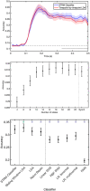
Classification accuracy achieved by different MVPA methods. Top panel: Plotting the accuracy (mean over subjects ± SE) versus time for STRM‐Classifier (with K optimised through cross‐validation—see Section 2) versus timepoint‐by‐timepoint spatially resolved decoding identify marginal improvements in classification accuracy over later timepoints when temporal patterns are identified. Middle panel: Plots of mean accuracy over all timepoints between 0 and 0.5 s as a function of the number of states K; plot shows mean over subjects ± SE. This shows this relationship is robust for values of the parameter K above a sufficient level; equivalent decoding accuracy is achieved when using K = 10 states or higher. Lower panel: the STRM‐Classifier performs favourably when compared with discriminative classification methods. We here compare the STRM classifier with eight other classification methods—three other spatially resolved classifiers (LDA with optimised sliding window length—see Section 2; LDA using the conventional timepoint‐by‐timepoint decoding approach, and Naive Bayes using the conventional timepoint‐by‐timepoint decoding approach); and additionally five different discriminative classifiers fit using timepoint‐by‐timepoint methods (Linear SVMs, non‐linear SVMs using a radial basis function (RBF) kernel; binomial and multinomial logistic regression (LR), and K‐nearest neighbour (KNN) classifiers with K optimised through cross‐validation). We find in general that generative encoding model based classifiers (STRM, LDA and Naive Bayes) outperform discriminative classifiers (SVM, LR and KNN), and furthermore that STRM decoding outperforms equivalent methods when used with the conventional timepoint‐by‐timepoint decoding approach; however, we similarly find that these gains are slightly surpassed by optimised sliding window methods. Asterisks denote significantly different from STRM‐Classifier accuracy at Bonferroni corrected levels; green asterisks show significantly higher accuracy (Sliding Window LDA); blue significantly lower (all other classifiers)

FIGURE 5

Resolving the successive stages of visual stimulus processing in space and time. Fitting the STRM‐Classification model independently to each subject's MEG data recorded during visual stimulus presentation, using K = 8 states allows us to investigate the stages of visual stimulus processing and the times on individual trials at which they emerge, subject to the usual interpretational caveats associated with the inverse problem and loss of information content in our source reconstruction methods. Top panel: Average timing of each state over a trial (mean ± SE over subjects), demonstrating the mean time after stimulus presentation that each state emerges. Lower central panel: a raster plot of state timecourses inferred for a sample subject over 248 trials, demonstrating the variability in timings over successive trials within the common left‐to‐right HMM pattern progressing from state 1 to 8. Lower outer panels: the thresholded, group‐mean f statistics, per ROI, as a result of multiple subject‐level ANOVAs; this displays the amount of information contributed by that ROI to discriminate the different visual stimuli (see Section 2). Statistics are thresholded at the 75th percentile of all test statistics obtained

FIGURE 6

The timing of visual processing is modulated by behaviour and physiology. Panel a: inter‐stimulus intervals do not significantly modulate state transition times. Panel b: Longer participant reaction times are predictive of delayed transitions into states 3–8, with increasing effect size toward later states. Panel c: increases in baseline broadband power are associated with more rapid transitions into state 2, an early visual processing state. Panel d: increases in baseline alpha power over visual areas is associated with delayed transitions from state 4 into state 5. In all bar plots, asterisks denote significance at Bonferroni corrected levels (p = 2.1e − 3)

FIGURE 7

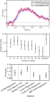
Predictive accuracy of STRM‐Regression decoding Top panel: plotting the Pearson correlation between model predictions and true regressor values over time, we see equivalent performance by both metrics. The STRM‐Regression output shown here was obtained by optimising the value of K (the number of states) by subject‐level cross‐validation (see Section 2). Middle panel: this performance is robust over a range of values for the parameter K controlling the number of states, with STRM‐Regression displaying no significant difference from synchronous models for all values of K tested (ANOVA, p = .98); this plot does further identify a performance tuning curve that justifies the use of optimisation through cross‐validation. Lower panel: Performance of STRM‐Regression against a range of different decoding models, both generative (LGS—in both synchronous and optimised sliding window modes) and discriminative (linear regression and Support vector machine regression, using linear and radial basis function kernels). The Pearson correlation shows no significant difference between groups (ANOVA; p = .19). While not significant, the trend is the same as obtained for STRM‐classification: STRM‐Regression is broadly consistent in performance with its timepoint‐by‐timepoint LGS equivalent, however optimised sliding window methods are trending toward superior performance than STRM‐Regression. There is no evidence that discriminative models (Linear Regression and SVM regression) in general outperform generative models (LGS and STRM), with the results here trending in the other direction

FIGURE 8

The stages of EEG Value Processing. Fitting the STRM‐Regression model independently to each subject's EEG data with K = 8 states identified a consistent pattern of sequential activity on each trial, but with significant variation in the timing of events on individual trials. Top panel: mean state timecourse ± SE over subjects. Lower centre panel: example state timecourses for one subject exhibiting significant variation over trials. Lower outer panels: Mean (over subjects) activation patterns for each state and each regressor. Each trial is associated with consistent patterns of activity, comprising a mean pattern of activation common to that stage of cognitive processing on all trials and a separate value‐specific component. Both components are characterised by medial parietal activation; in the case of the value signal this appears to emerge initially in parietal areas (e.g., state 2) and later move to more frontal regions (state 6). In response to concerns about eye movement artefacts accounting for significant decode‐ability, none of these topographies appears eye movement related

FIGURE 9

The timing of value processing is modulated by cognitive variables. We investigated whether latent cognitive variables within the overall task structure significantly affected the timing at which different stages of value processing emerged on different trials. Specifically, we asked whether three regressors—the overall reward accumulated, the accrual time, and the recent reward rate—could predict the transition times between states on individual trials. We found no significant effect of reward accumulated, the variable being decoded, however we found significant effects of accrual times (reflecting how much time the participant invested to obtain the reward) and recent reward history (reflecting the expected value of alternative sites). Longer accrual times were associated with more rapid transitions through early stimulus processing states, whereas high rewards in recent history were associated with delayed transitions into intermediate stimulus processing states

References

1. Anderson, J. R. , Betts, S. , Ferris, J. L. , & Fincham, J. M. (2010). Neural imaging to track mental states while using an intelligent tutoring system. Proceedings of the National Academy of Sciences of the United States of America, 107(15), 7018–7023. 10.1073/pnas.1000942107 - DOI - PMC - PubMed
1. Anderson, J. R. , & Fincham, J. M. (2014a). Discovering the sequential structure of thought. Cognitive Science, 38(2), 322–352. 10.1111/cogs.12068 - DOI - PubMed
1. Anderson, J. R. , & Fincham, J. M. (2014b). Extending problem‐solving procedures through reflection. Cognitive Psychology, 74, 1–34. 10.1016/j.cogpsych.2014.06.002 - DOI - PubMed
1. Anderson, J. R. , Fincham, J. M. , Schneider, D. W. , & Yang, J. (2012). Using brain imaging to track problem solving in a complex state space. NeuroImage, 60(1), 633–643. 10.1016/j.neuroimage.2011.12.025 - DOI - PMC - PubMed
1. Beal, M. J. (2003). Variational algorithms for approximate bayesian inference (PhD Thesis [Issue May]). Gatsby Computational Neuroscience Unit, University College London.
Publication types