The interplay of additivity, dominance, and epistasis on fitness in a diploid yeast cross

Abstract

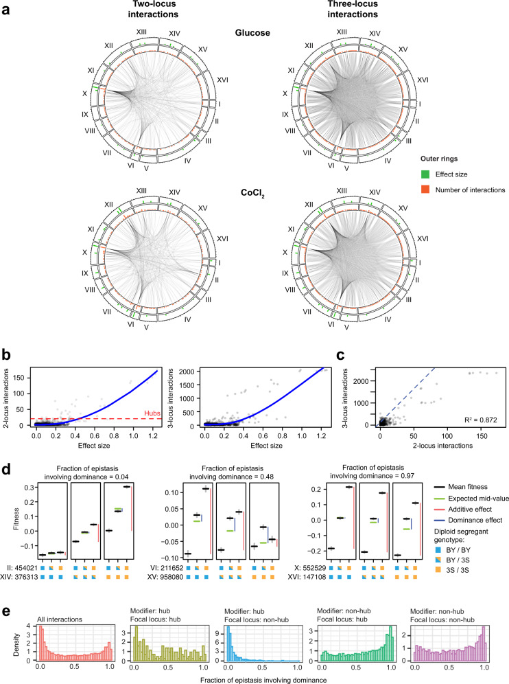
In diploid species, genetic loci can show additive, dominance, and epistatic effects. To characterize the contributions of these different types of genetic effects to heritable traits, we use a double barcoding system to generate and phenotype a panel of ~200,000 diploid yeast strains that can be partitioned into hundreds of interrelated families. This experiment enables the detection of thousands of epistatic loci, many whose effects vary across families. Here, we show traits are largely specified by a small number of hub loci with major additive and dominance effects, and pervasive epistasis. Genetic background commonly influences both the additive and dominance effects of loci, with multiple modifiers typically involved. The most prominent dominance modifier in our data is the mating locus, which has no effect on its own. Our findings show that the interplay between additivity, dominance, and epistasis underlies a complex genotype-to-phenotype map in diploids.

Fig. 1. Generating a large panel of diploid segregants with known genotypes that can be phenotyped as a pool.

a Overview of the experimental design. Parental haploids, BY and 3S, were mated and sporulated. The resulting MATα and MATa segregants were barcoded at a common genomic location and sequenced. Segregants were mated as pairs to generate a panel of ~200,000 double-barcoded diploid strains with known genotypes. All diploid strains originating from a single haploid parent are referred to as a ‘family’. b MATα and MATa barcodes were brought to the same genomic location by inducing recombination between homologous chromosomes via Cre-loxP. c Diploid strains were pooled and grown in competition for 12–15 generations. Barcode sequencing over the course of the competition was used to estimate the fitness of each strain. d Density plot of the raw fitness of double barcodes representing the same diploid strain in the same pooled growth condition (Glucose 1). e Density plot of the mean raw fitness of the same diploid strain measured in two replicate growth cultures (Glucose 1 and Glucose 2). f The mean broad-sense and narrow-sense heritability estimates for the 8 environments. The standard errors for both heritability estimates are shown as error bars for each point. g Violin plots of the fitnesses of diploid strains in 8 environments (n > 187,000 in each environment). Raw fitness estimates of BY/BY, BY/3S, 3S/BY, and 3S/3S diploid strains are shown as colored lines. Overlaid boxplots, here and in subsequent figures, indicate the median (white dots), interquartile range (IQR; black boxes), and lower and upper adjacent values (black lines extending from the black boxes), defined as first quartile − 1.5 IQR and third quartile + 1.5 IQR, respectively.

Fig. 2. Identification of loci that affect fitness.

a, b Loci mapped in CoCl₂ (a) and CuSO₄ (b). Panels from top to bottom are (1) loci detected using the mixed effects linear model FaST-LMM (red bars), (2) loci with dominance effects detected using a fixed effects linear model on the non-additive portion of each diploid’s phenotype (green bars), (3) loci enriched for detections in family-level scans (orange bars), (4) loci detected using family-tests (black or blue points), where each row is a different MATa family, and (5) the total number of detections across families for each 20 kb interval (gray bars). c Violin plot showing the % of loci that were detected in both glucose replicates for each family (n = 392 MATa families). d Scatterplot showing distinct loci detected using family-level tests with permutation-based thresholds in CoCl₂ and their maximal −log₁₀(p) values in each family in which they were identified. Red, green, and blue labels denote distinct loci in family-level scans that were also identified by FaST-LMM, dominance scans, or enrichment tests, respectively. Distinct loci showed substantial variability in statistical significance across families and mapping methods. e Barplot comparing the number of enriched family-level loci (red) and FaST-LMM loci (blue) detected across environments. Loci that were detected using both mapping methods are in dark colors, while loci that were specific to either FaST-LMM or family-level scans are in light colors. f Examples of loci with only additive effects (or low dominance), incomplete dominance, complete dominance, overdominance, and underdominance. All genotype classes had n > 41,000. Black lines are the mean fitness of diploids subsetted by the genotype state at the focal locus. Gray lines are the standard errors. Green lines are the expected mean fitness of heterozygotes assuming no dominance. Genotype state at each locus is denoted by colored boxes: BY/BY (blue), 3S/3S (orange), is BY/3S (half blue, half orange). Dominance and additive effects (blue and red bars, respectively) for each subset of the data are shown next to the relevant genotype classes. The degree of dominance at a locus is included in parentheses. g Violin plot showing the degree of dominance for all loci detected in the dominance scan (n = 142). Loci with positive values are dominant towards the allele conferring higher fitness (green), while loci with negative values are dominant towards the deleterious allele (red). All loci with degree of dominance >100% or < −100% exhibit overdominance and underdominance, respectively.

Fig. 3. Interactions often affect both the additive and dominance effects of involved loci.

a Interaction plots of all two-locus (left) and three locus (right) effects for two representative environments. Significant interactions between loci are shown as connecting lines. Green bars are the absolute effect size of a locus, calculated as the absolute difference between the mean fitness of diploids that are 3S/3S and BY/BY at the focal locus. Orange bars are the number of interactions detected for each locus. b Scatter plot of the absolute effect size of a locus and the number of two-locus (left) and three-locus (right) interactions in which it is involved. Local regressions are shown as blue lines. c Scatter plot of the number of two-locus and three-locus interactions per locus. d Examples of genetic interactions with, from left to right, low (0.04), moderate (0.48), and high (0.97) fractions of epistasis involving dominance. All genotype classes had n > 8,700. Black lines are the mean fitness of diploids subsetted by the genotype state at the two involved loci. Gray lines are the standard errors. Green lines are the expected mean fitness of heterozygotes assuming no dominance. Genotype state at each locus is denoted by colored boxes: BY/BY (blue), 3S/3S (orange), is BY/3S (half blue, half orange). The first locus is the locus whose effect is being modified, and the second locus is the modifier locus. Dominance and additive effects (blue and red bars, respectively) for each subset of the data are shown next to the relevant genotype classes. e Density plot of the fraction of epistasis involving dominance for all interactions (red; n = 3,522 genetic interactions), hub-hub (yellow; n = 87), non-hub-hub (blue; n = 2197), hub-non-hub (green; n = 2197), and non-hub-non-hub interactions (purple; n = 1,238).

Fig. 4. Multiple modifier loci cause hubs to exhibit a range of effect sizes across different genetic backgrounds.

a Specific examples of hubs on Chromosome VI, X, and XII (each row) and their additive (left) and dominance (right) modifiers. The height of the bar corresponds to the magnitude of the modifying effect. The dotted red line shows the threshold in which loci were considered as major effect modifiers. b Barplot showing the total number of times loci were detected as a major effect modifier of additive (left) or dominance (right) effects of hubs across environments. Colored dots indicate hub loci. An asterisk indicates a non-hub locus on ChrIII. c Additive (top; n > 443 for each genotype class) or dominance (bottom; n > 175 for each genotype class) effect size of Chromosome VI hub in NaCl across different allelic combinations of its four largest effect modifiers. Red points are the mean effect size of a genotype class based on the genotype state of the four modifiers. Black point is the overall mean effect size of the locus. Black lines are bootstrapped 95% confidence intervals.

Fig. 5. Parent-of-origin of the mating locus influences dominance at hubs.

a Violin plots of the fitness distribution of diploid strains split by the genotype at the Chromosome X locus (top), further split by the genotype at the mating locus on Chromosome III (middle), and the parent-of-origin at the mating locus (bottom). All genotype classes had n > 9000. Genotype state at each locus is denoted by colored boxes: BY/BY (blue), 3S/3S (orange), is BY/3S (half blue, half orange). Lines are the observed mean fitness in the homozygous genotype classes (gray), the observed mean fitness in heterozygous genotype classes (red), and the expected heterozygous fitness if there was no dominance (blue). b Violin plots of the fitness distribution of diploid strains split by the genotype state of a hub locus and the parent-of-origin of the mating locus: Chromosome VI hub (top), Chromosome XII hub (middle), Chromosome XIV hub (bottom). All genotype classes had n > 9500.

References

1. Mackay TFC, Stone EA, Ayroles JF. The genetics of quantitative traits: challenges and prospects. Nat. Rev. Genet. 2009;10:565–577. - PubMed
1. Bloom JS, Ehrenreich IM, Loo WT, Lite T-LV, Kruglyak L. Finding the sources of missing heritability in a yeast cross. Nature. 2013;494:234–237. - PMC - PubMed
1. Boyle EA, Li YI, Pritchard JK. An expanded view of complex traits: from polygenic to omnigenic. Cell. 2017;169:1177–1186. - PMC - PubMed
1. Shao H, et al. Genetic architecture of complex traits: Large phenotypic effects and pervasive epistasis. Proc. Natl Acad. Sci. USA. 2008;105:19910–19914. - PMC - PubMed
1. Mackay TFC. Epistasis and quantitative traits: using model organisms to study gene–gene interactions. Nat. Rev. Genet. 2014;15:22–33. - PMC - PubMed
Publication types
LinkOut - more resources