. 2022 Mar 2:15:749728.
doi: 10.3389/fnins.2021.749728. eCollection 2021.

Stochastic Motion Stimuli Influence Perceptual Choices in Human Participants

Affiliations

Stochastic Motion Stimuli Influence Perceptual Choices in Human Participants

Pouyan R Fard et al. Front Neurosci. .

Abstract

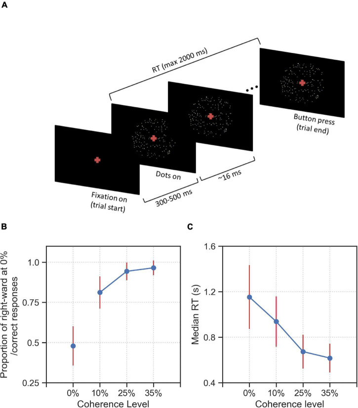
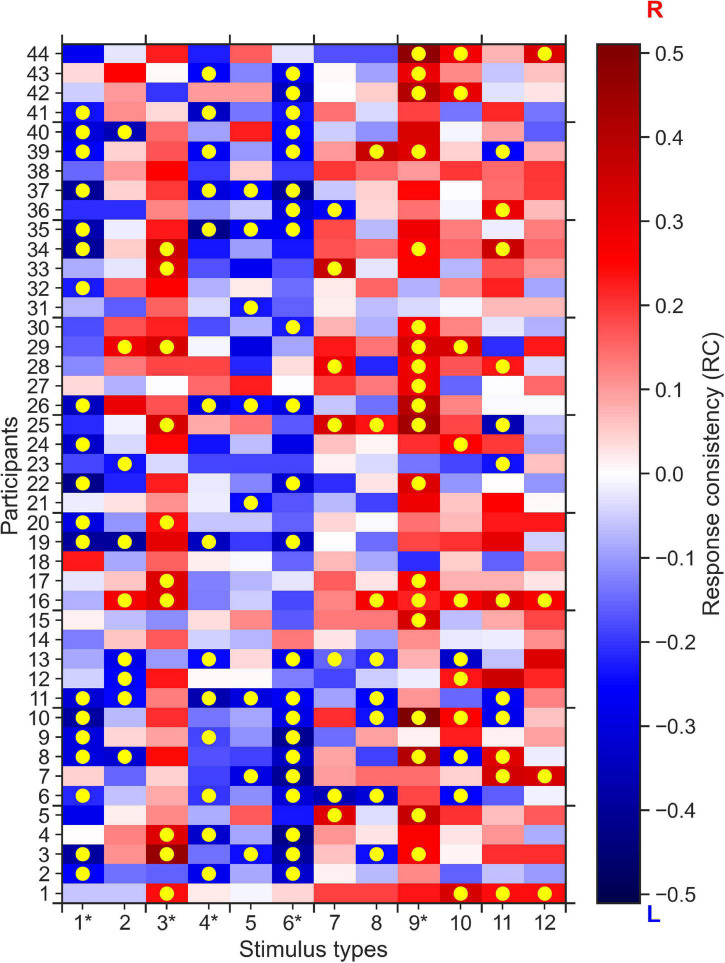
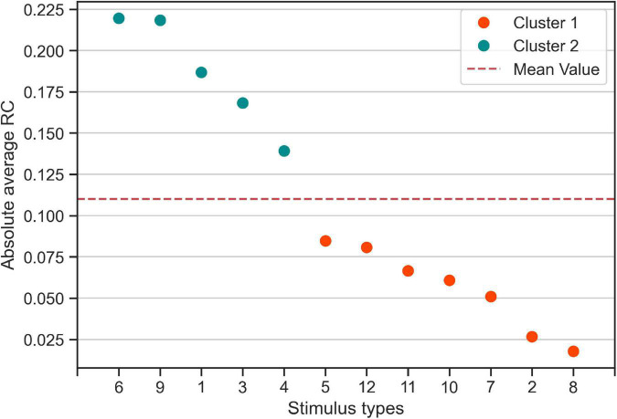
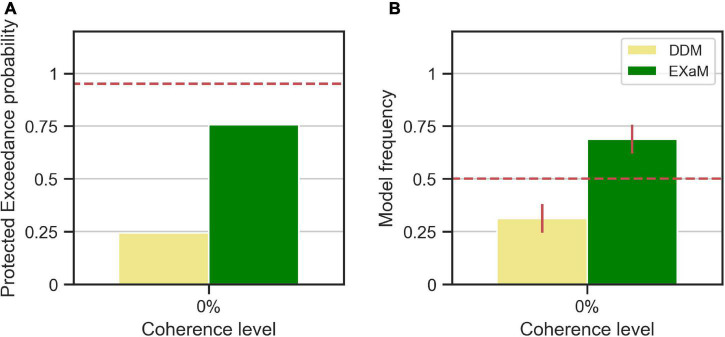
In the study of perceptual decision making, it has been widely assumed that random fluctuations of motion stimuli are irrelevant for a participant's choice. Recently, evidence was presented that these random fluctuations have a measurable effect on the relationship between neuronal and behavioral variability, the so-called choice probability. Here, we test, in a behavioral experiment, whether stochastic motion stimuli influence the choices of human participants. Our results show that for specific stochastic motion stimuli, participants indeed make biased choices, where the bias is consistent over participants. Using a computational model, we show that this consistent choice bias is caused by subtle motion information contained in the motion noise. We discuss the implications of this finding for future studies of perceptual decision making. Specifically, we suggest that future experiments should be complemented with a stimulus-informed modeling approach to control for the effects of apparent decision evidence in random stimuli.

Keywords: Bayesian inference; drift-diffusion model; model comparison; perceptual decision making; random-dot motion task.


Conflict of interest statement

The authors declare that the research was conducted in the absence of any commercial or financial relationships that could be construed as a potential conflict of interest.

Figures

FIGURE 1
FIGURE 1
Experimental design and behavioral results on group level. (A) a fixation cross was shown for a variable duration between 300 and 500 ms. After this fixation period, a cloud of ∼40 dots appeared within an aperture of 12 degrees on the center of the screen. In each trial, a proportion of all dots shown, as indicated by the coherence level, were moving toward the direction (right or left) indicated by the trial-wise target alternative. The remaining dots were displaced randomly within the aperture. Dot positions were updated every 16 ms. The trial ended when the participant makes a decision (button press) or a maximum of 2,000 ms has elapsed from the onset of the first frame of dots. The task was to decide into which of two directions the dots were moving (left or right). (B) Proportion correct (or proportion of rightward responses for 0% coherence stimuli) and (C) median RT averaged over all 44 participants for the four coherence levels (0%, 10%, 25%, and 35%). Error bars indicate the standard deviation across all participants, excluding the timed-out trials.
FIGURE 2
FIGURE 2
0% coherence trials: Response consistency (RC) map across 44 participants and 12 stimulus types. Positive RC values (red) report the tendency of a participant to choose the rightward direction, whereas the negative RC values (blue) report the tendency for the left direction. Yellow circles indicate significantly (p < 0.05, corrected for number (12) of stimulus types) consistent right (dark-red) and left (dark-blue) responses of a specific participant, across up to 20 repetitions of a specific stimulus type. One can clearly see that for stimulus types 1, 3, 4, 6, and 9 (indicated by an asterisk), most participants have mostly the same consistent responses, e.g., we see mostly red colors for stimulus type 9, i.e., the participants tend to respond right more than they do overall.
FIGURE 3
FIGURE 3
Categorization of stimulus types based on absolute average response consistency (RC) values. Using the absolute of the RCs averaged across participants, we used K-means clustering to categorize the twelve 0% coherence stimulus types according to consistency averaged over participants. Cluster 1 (Orange) contains seven stimulus types for which participants made responses that are less consistent than the average (red dashed line). Cluster 2 contains the five stimulus types to which participants responded more consistently than on average.
FIGURE 4
FIGURE 4
Results of random-effects Bayesian model comparison between DDM and EXaM for 0% coherence across 44 participants, (A) Protected exceedance probability (probability that a model is the best model for all participants). The red dashed line indicates very strong evidence for a model (0.95). (B) Model frequency, i.e., the probability that a randomly selected participant’s behavior is best explained by the specific model. The red dashed line represents chance level and error bars indicate the standard deviation of the estimated model frequencies.
FIGURE 5
FIGURE 5
Results of random-effects Bayesian model comparison for zero % coherence level across two groups of participants; (A) the observed model comparison results in Figure 4 are actually driven by the high-performing participants. The left plot shows the protected exceedance probability (probability that a model is the best model for all participants). The red dashed line indicates very strong evidence for a model (0.95). The right plot shows the model frequency for model comparison between DDM and EXaM. The model frequency is the probability that the behavior of a randomly selected participant is best explained by a specific model, among the compared models. The red dashed line represents chance level and error bars indicate the standard deviation of the estimated model frequencies. (B) The same plots as in A for the low-performing participants.
FIGURE 6
FIGURE 6
The relationship between zero % coherence response consistency and average posterior estimates of the EXaM’s scale parameter. The average posterior scale estimate for Cluster 2 stimulus types (sc¯2) is plotted as a function of average absolute RC across Cluster 2 stimulus types. The regression line shows a positive correlation between two variables (linear regression Eq. 2, R = 0.34, p < 0.05). The data from two participants was excluded as their sc¯2 values were outliers.
FIGURE 7
FIGURE 7
Determining the consistent responses given the response bias (right) of the participants; the rightward responses bias for each participant (A) is used to create the null hypothesis distribution of frequency of rightward responses (blue histogram) for each participant (B–D, for three exemplary participants). The null hypothesis distribution (the blue histogram) is binomial distribution centered on the rightward response bias of the participant (red dashed line). If the participant is in general unbiased toward right or left alternatives, then the null hypothesis distribution is centered around 10 (as in B), i.e., half of the maximum number of responses for each stimulus type (20). If the participant is in general biased toward right (C) or left (D) the mean value of the null hypothesis is shifted toward 20 or 0, respectively. The null hypothesis distribution is used to determine the whether the observed frequency of rightward responses of the participant to a specific stimulus type (two exemplary pink stars for two different stimulus types) is consistent. If an observed frequency is extreme enough w.r.t. to mean of the null hypothesis distribution, then the response of the participant to that stimulus type is consistent. For example, the observed rightward frequency of 16 is consistent in (B,D), but not in (C). Likewise, the observed rightward frequency of 4 is consistent in (B,C), but not in (D).
FIGURE 8
FIGURE 8
The dot counting algorithm and stimulus features. (A) Schematic of dot counting algorithm: the algorithm iterates through every dot within the stimulus aperture at every time-step, t. If within a time period of 50 ms (up to three frames) after t there exists a dot within a square area to the right of the current dot (red area), the dot movement is rightward (green arrow to a yellow dot within the red area) and the dot counts (DC) for the respective time-step, dc(t), is incremented. Likewise, if within the similar time period there exists a dot within the area to the left of the current dot (blue area), the dot movement is leftward (indicated by green arrow to the yellow dot within the blue area) and the dc(t) is decremented. The dot movements outside of the red and blue areas (indicated by orange arrows) dot not contribute to the value of dc(t) for the dot currently being considered, (B) a representative example time-course of the computed DC for a single trial with 0% coherence stimulus type 6. The labels R and L indicate the directions encoded by the DC features. (C) Average normalized DC values shown as a function of coherence level and trial-wise direction of correct alternative. The normalized DC values are computed as the DC values divided by the standard deviation of absolute dot count values across all trials containing stimuli of the same coherence level. The average value of normalized DC is then computed across all trials related to the coherence level with the respective direction of correct alternative (right or left). Error bars indicate the standard error of the mean.
FIGURE 9
FIGURE 9
Visualization of parameter distributions. (A) Prior densities for each parameter in Table 3, (B) Example (marginal) posterior parameter densities of the EXM for participant 44, 0% coherence level.

Similar articles

References

    1. Adelson E. H., Bergen J. R. (1985). Spatiotemporal energy models for the perception of motion. J. Opt. Soc. Am. A 2 284–299. 10.1364/josaa.2.000284 - DOI - PubMed
    1. Bair W., Koch C. (1996). Temporal precision of spike trains in extrastriate cortex of the behaving macaque monkey. Neural Comput. 8 1185–1202. 10.1162/neco.1996.8.6.1185 - DOI - PubMed
    1. Barthelmé S., Chopin N. (2013). Expectation propagation for likelihood-free inference. J. Am. Stat. Assoc. 109 315–333. 10.1080/01621459.2013.864178 - DOI
    1. Benjamini Y., Hochberg Y. (1995). Controlling the false discovery rate – a practical and powerful approach to multiple testing. J. R. Stat. Soc. Ser. B Methodol. 57 289–300. 10.1111/j.2517-6161.1995.tb02031.x - DOI
    1. Britten K. H., Newsome W. T., Shadlen M. N., Celebrini S., Movshon J. A. (1996). A relationship between behavioral choice and the visual responses of neurons in macaque MT. Vis. Neurosci. 13 87–100. 10.1017/s095252380000715x - DOI - PubMed

LinkOut - more resources