Spatial transcriptomic reconstruction of the mouse olfactory glomerular map suggests principles of odor processing

Abstract

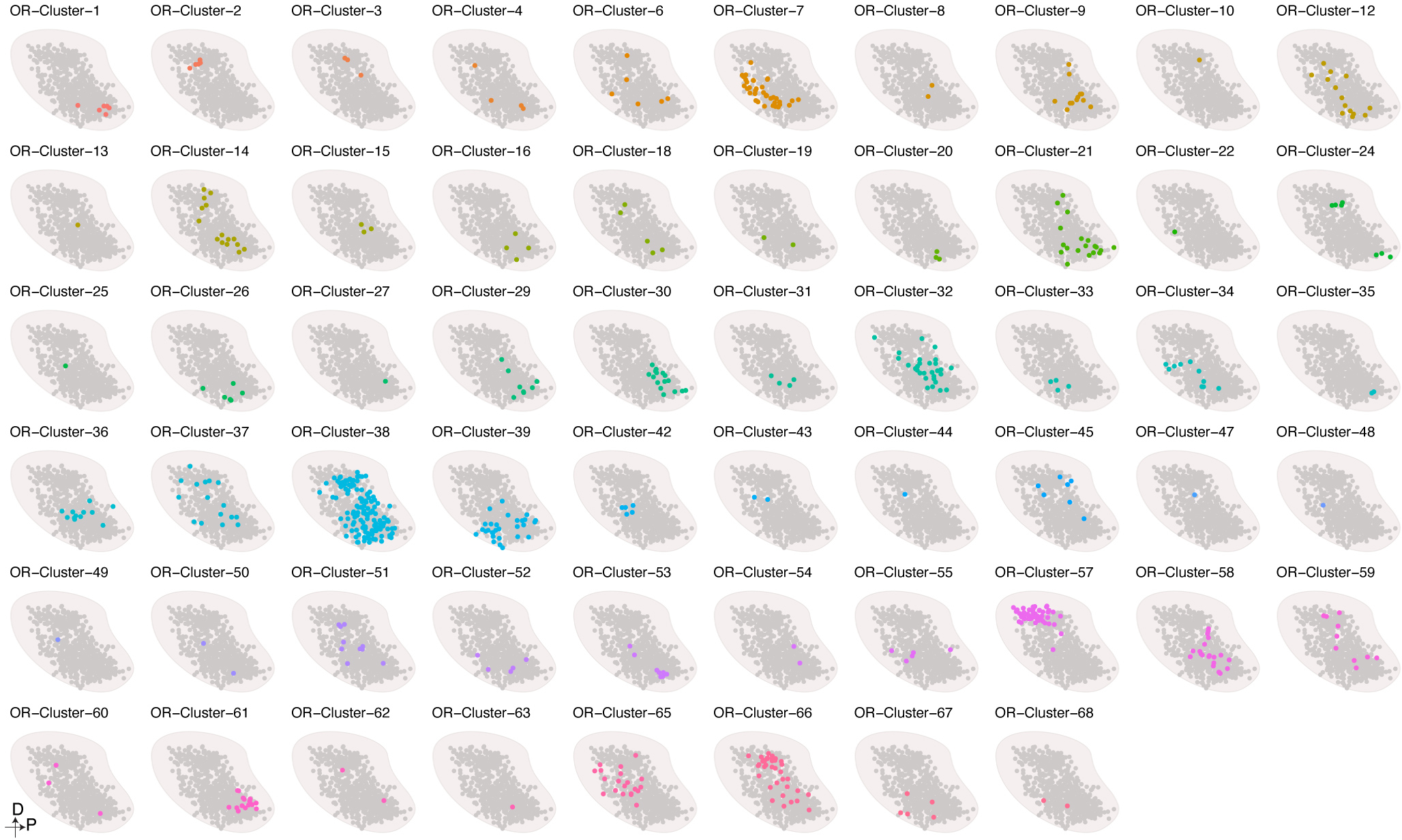
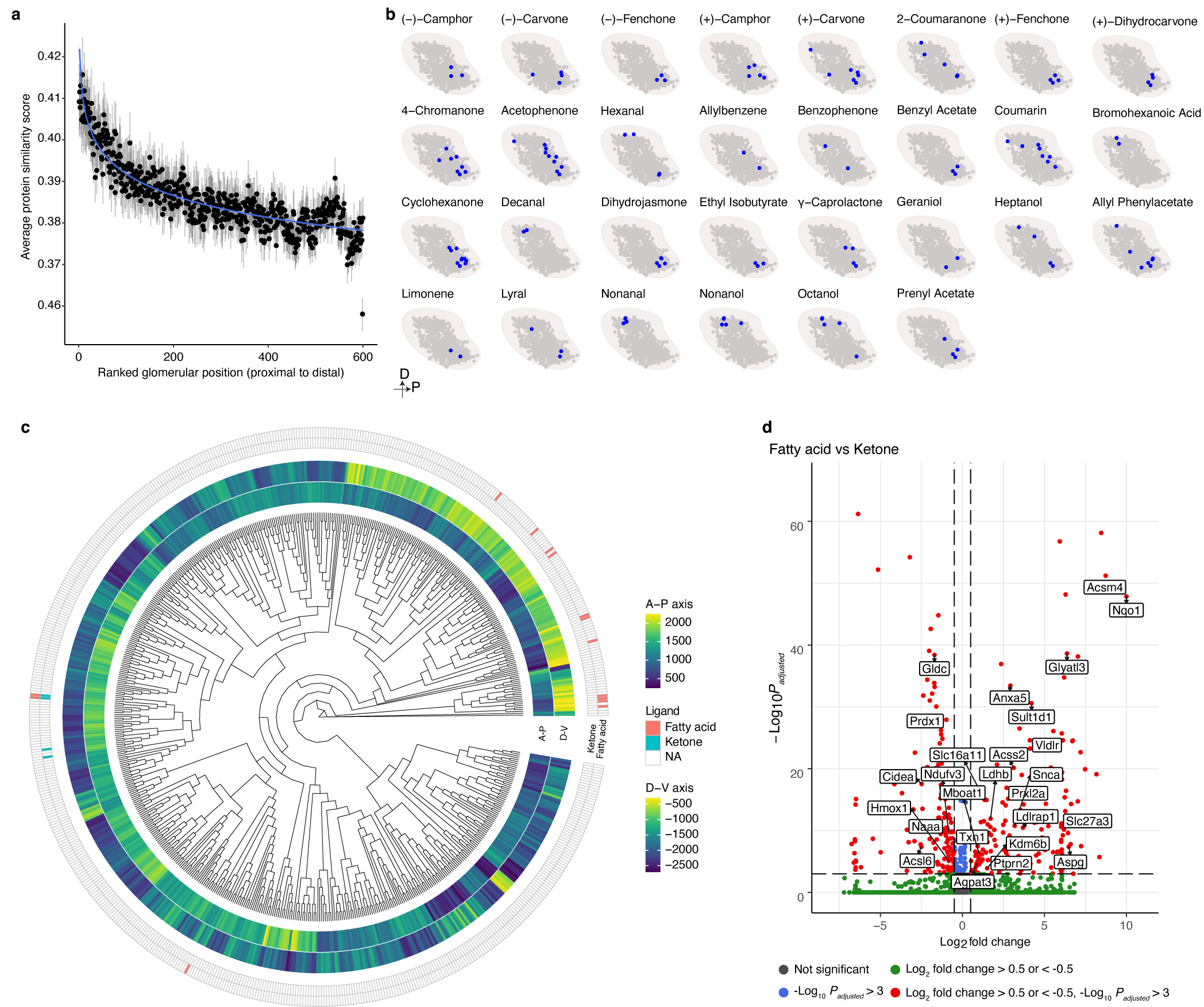
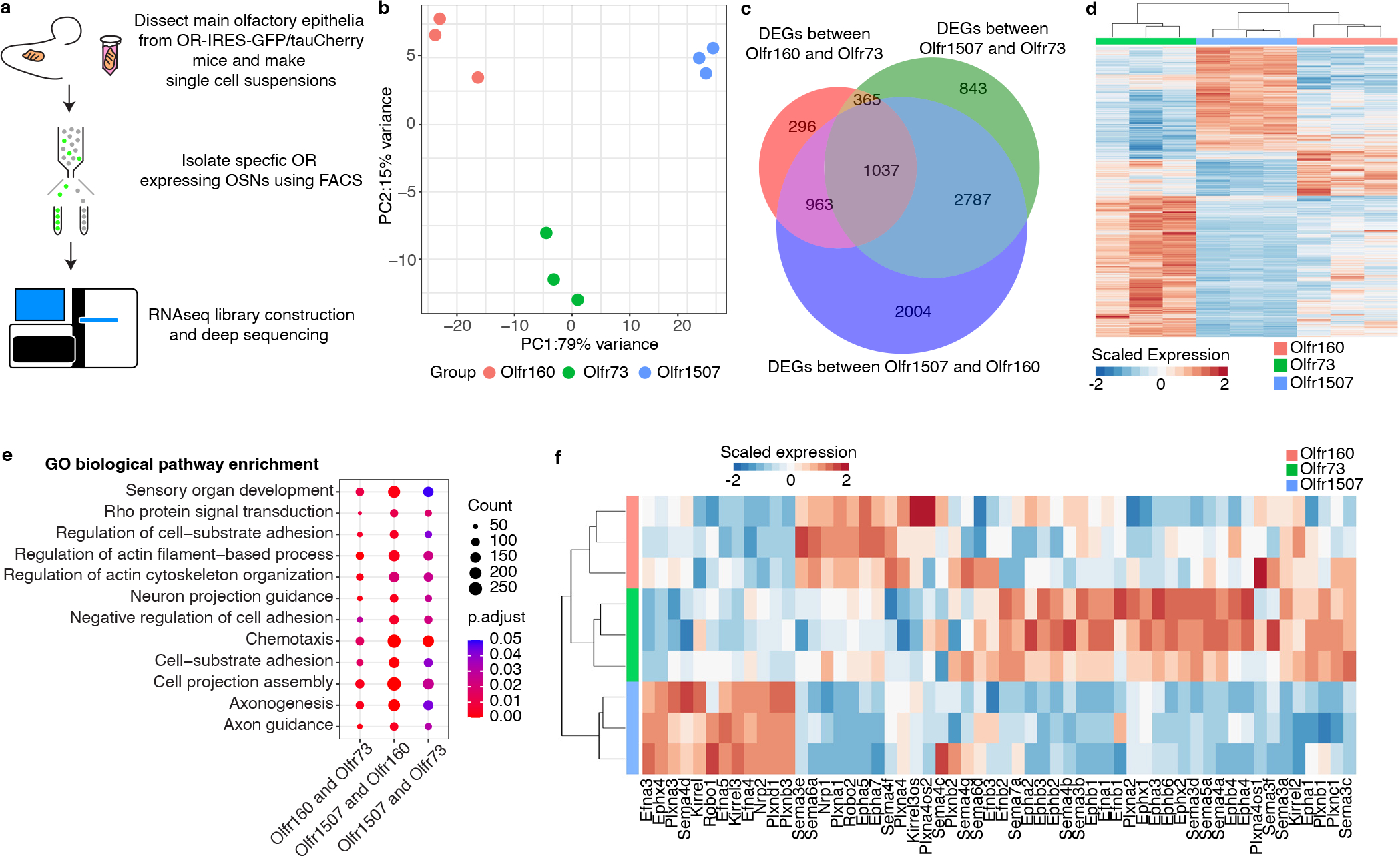
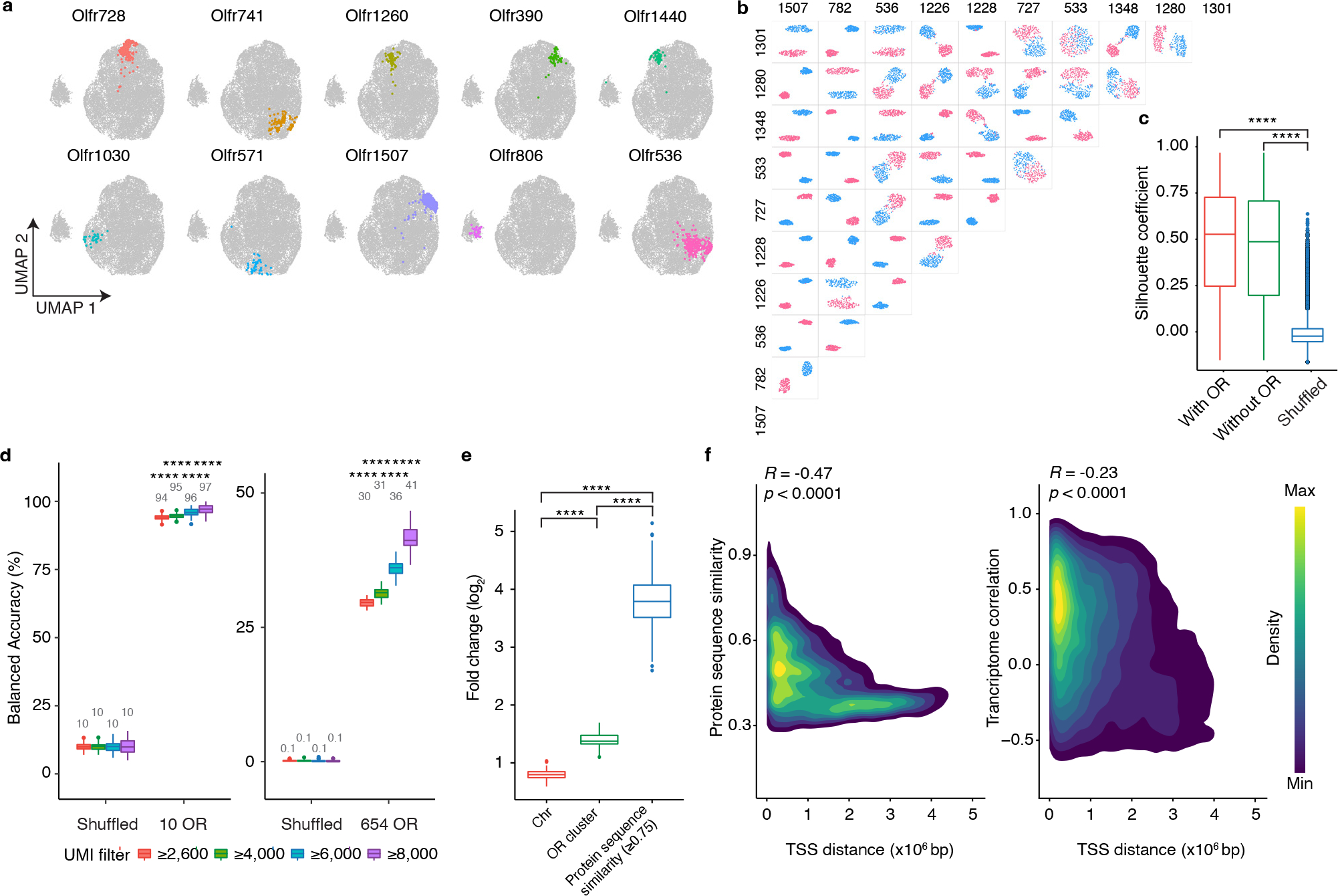
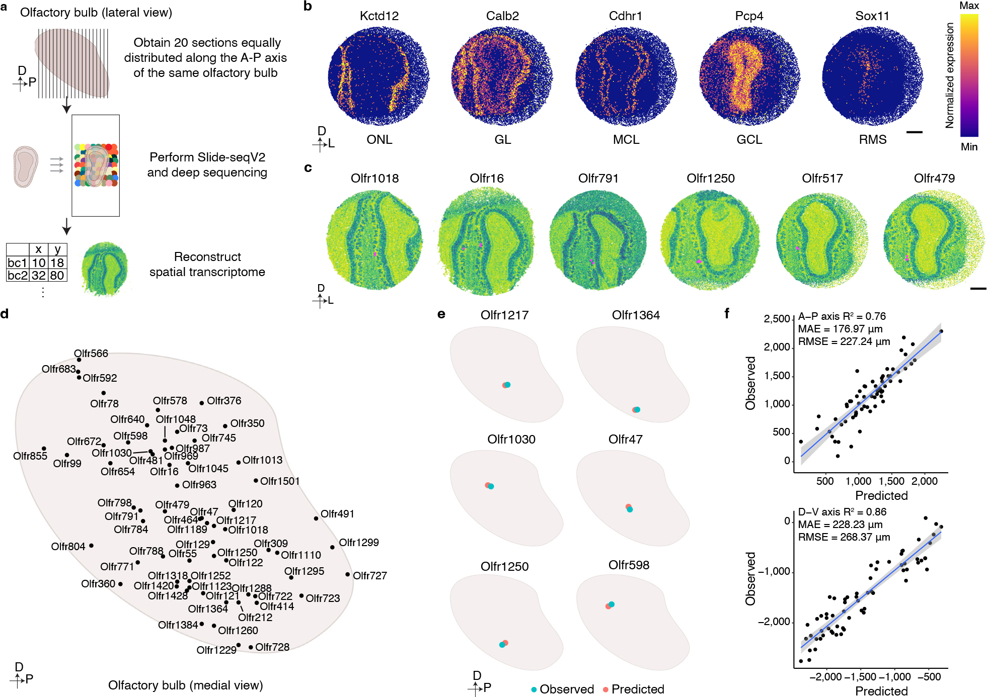
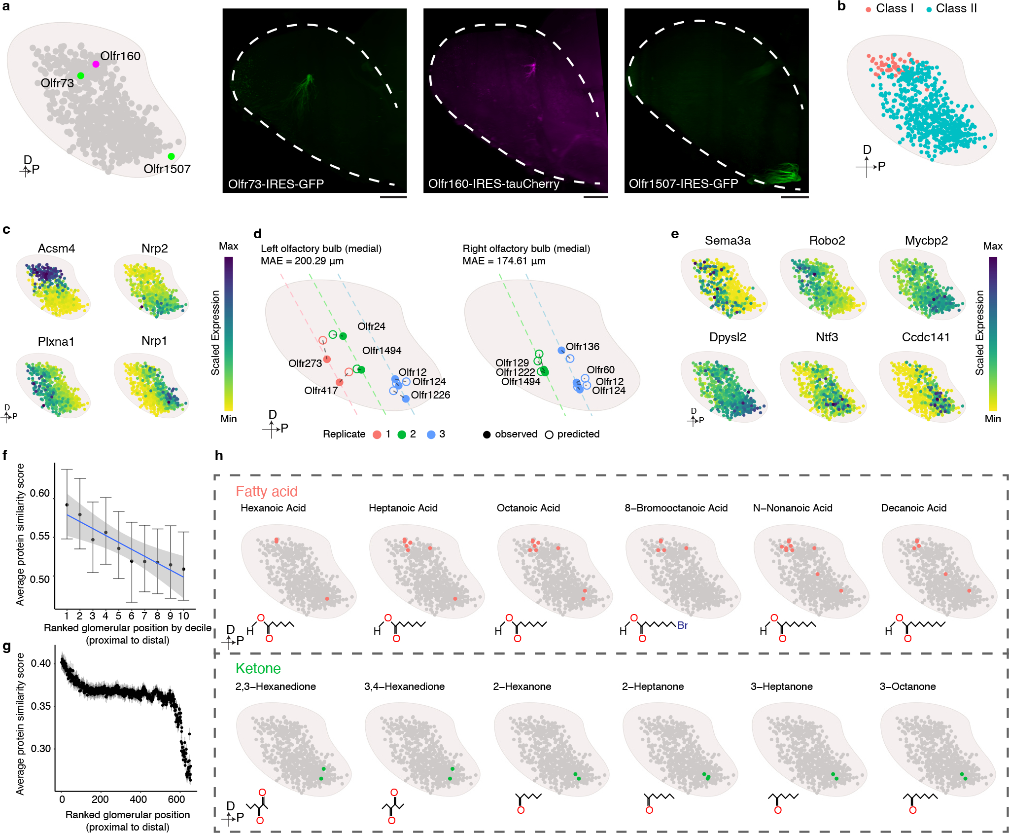
The olfactory system's ability to detect and discriminate between the vast array of chemicals present in the environment is critical for an animal's survival. In mammals, the first step of this odor processing is executed by olfactory sensory neurons, which project their axons to a stereotyped location in the olfactory bulb (OB) to form glomeruli. The stereotyped positioning of glomeruli in the OB suggests an importance for this organization in odor perception. However, because the location of only a limited subset of glomeruli has been determined, it has been challenging to determine the relationship between glomerular location and odor discrimination. Using a combination of single-cell RNA sequencing, spatial transcriptomics and machine learning, we have generated a map of most glomerular positions in the mouse OB. These observations significantly extend earlier studies and suggest an overall organizational principle in the OB that may be used by the brain to assist in odor decoding.

Extended Data Figure 1:. FACS isolation of specific OR-expressing OSNs using OR-IRES-GFP/mCherry knockin mice.

a, Scatter plots of FACS isolated, dissociated olfactory epithelial cells from mice harboring the Olfr160-IRES-tauCherry (top), the Olfr73-IRES-GFP (middle), or the Olfr1507-IRES-GFP (bottom) alleles. The gate used to isolate ~100% pure populations of fluorescent OSNs is indicated. b, Mature OSN markers (e.g., Omp and Cnga2) but not immature OSN markers (e.g., Gap43) are detected in FACS isolated samples. c, Each OSN population selectively expresses its corresponding OR.

Extended Data Figure 2:. scRNAseq reveals diverse cell types in the main olfactory epithelium.

a, Schematic representation of the workflow used to perform scRNAseq on cellular populations isolated from the mouse main olfactory epithelium. b, The distribution of different cell types on the UMAP projection plots. HBC: horizontal basal cell; GBC: Globose basal cell; INP: Immediate neuronal precursor; iOSN: immature olfactory sensory neuron; OSN: Olfactory sensory neuron; MV: Microvillar cell; SUS: Sustentacular cell; BG: Bowman’s gland; OEC: Olfactory ensheathing cell; EC: Ependymal cell; MC: myeloid cell; MP: Macrophage; BC: B cell; TC: T cell; NP: Neutrophil; NKN: Unknown. c, Violin plots of the genes used to assign cell types. d, Dot plot of a subset of the differentially expressed genes between cell types. For each gene depicted, the size of the circle corresponds to the percentage of sequenced cells in which transcripts that map to that gene were detected, and the color reflects the average expression level of the gene within those cells.

Extended Data Figure 3:. Quality control analysis of OSN scRNAseq.

a, Histogram of the number of distinct OR expressed by each of the mature OSNs captured in scRNAseq experiments. b, Histogram of the number of UMIs detected by each of the single OR expressing OSNs captured in scRNAseq experiments, the cells with 15000 > UMI > 2600 were used for the future analyses (blue area). c, Plot of the number of cells sequenced that express each distinct OR, the OR transcript detected by Slide-seqV2 are labeled. Data are plotted as mean +/− SD from six independent experiments. d, Schematic of each cluster of OR genes and their chromosomal location and how many cells were detected that express each of these ORs.

Extended Data Figure 4:. UMAP projections reveal distinct transcriptomes expressed by different types of OSN.

a, Normalized expression of the Acsm4, Nrp2, Plxna1, and Nrp1 genes on UMAP projection plots of OSN scRNAseq data. b, UMAP plots of OSNs were regenerated with all OR gene expression information removed. OSNs expressing each of ten random ORs selected in Fig.2a are pseudo colored in the UMAP plot, revealing that cells displaying the same OR cluster together even in the absence of OR gene expression information. c, UMAP plots were regenerated in a pairwise manner using each of the groups of OSNs expressing the ten most frequently occurring ORs with OR gene expression information removed prior to clustering. In each pairwise analysis all of the OSNs expressing one OR are colored red, and all of the OSNs expressing the other OR are colored blue to make it easier to visualize their separation in UMAP space. d, “Shuffled” control for the pairwise OSN UMAP segregation analysis. The analysis was performed as in c, except OR identity was randomly assigned prior to analysis. e, Analysis of all of the differentially expressed genes identified in a pairwise manner for each of the 654 types of OSN. For each differentially expressed gene, we determined for each of the 654 types of OSN in how many of those types of OSN is that gene detected in at least 10% of the sequenced cells.

Extended Data Figure 5:. Pairwise analysis reveals OSN features that correlate with transcriptomic similarity.

a, Analysis of the ability to predict OR identity using different GO biological pathway term gene sets. The boxplots depict the bootstrapped data from 100 iterations of the prediction for each GO term, The top 30 terms are ordered from the highest mean accuracy to the lowest. In addition to the GO terms found in the axon guidance biological category, we hand curated a list of axon guidance genes and adhesion molecules (Supplementary Table 2), removing transcription factors and odorant receptor genes themselves and included this refined set of axon guidance/adhesion molecule genes in the analysis. b, Analysis of the ability to predict OR identity using different GO molecular pathway term gene sets. The boxplots depict the bootstrapped data from 100 iterations of the prediction for each GO term, The top 30 terms are ordered from the highest mean accuracy to the lowest. c, Incorrectly predicted ORs are likely to possess similar protein sequence to the correct OR. The OR protein similarity scores of incorrectly predicted OR pairs from Fig.2d were calculated and binned (N = 100 independent tests). The boxplot depicts the likelihood of a given OR protein similarity score distribution as the fold-change relative to random OR pairs. d, The transcriptomic correlation between a pair of OSNs positively correlates with the protein sequence similarity of the ORs they express. Transcriptomic correlation and OR protein sequence similarity of all the pairwise combination of 654 types of OSN were calculated and binned. The plot depicts the mean +/− SEM for each protein similarity score bin. e, Heat map of each set of OSNs expressing a specific OR reveals high transcriptional correlation (upper triangle) and OR protein sequence similarity (lower triangle) between OSNs expressing ORs located within the same genomic cluster. OSNs are ordered by genomic location and the color bar indicates the genomic cluster. Boxplots in this figure represent Q1–1.5*IQR, Q1, median, Q3, and Q3+1.5*IQR, data beyond the whisker were plotted as individual dots.

Extended Data Figure 6:. Slide-seqV2 enables high quality spatial transcriptomic analysis of the mouse OB.

a, Plot of the number of genes (left panel) or UMIs (right panel) detected per bead on each slide of the Slide-seqV2 experiments (N ranges from 30041 to 56016, the exact number of beads on each individual slide is provided in Supplementary data 1), Boxplots indicate Q1–1.5*IQR, Q1, median, Q3, and Q3+1.5 *IQR; data beyond the whisker were plotted as individual dots. b, Mitochondrial transcript levels as a marker to define layer organization in the OB. Scale bar: 500 μm. c, Schematic of automated calling of glomerular positions in Slide-seqV2 experiments. d, Slide-seqV2 identified glomerular positions match glomerular positions that have been empirically determined. Scale bar: 500 μm. e, The glomerular positions of 14 ORs detected in two replicates of 20 Slide-seqV2 experiments exhibit high spatial correlation. 13 of the 14 glomerular positions identified in two, independent biological replicates were used as the anchors to align the two OBs. The held-out glomerulus was then transformed based on the anchors and the position was recorded. This process was iterated for all 14 glomeruli. The correlation between the position of the held-out glomeruli on the A-P and D-V axes across both replicates is shown. Data were fitted with a regression line (blue), +/− 95% CI (light blue).

Extended Data Figure 7:. Validation of the predicted glomerular map.

a, Light sheet microscopic images of intrinsic fluorescent signals from the OBs of three independent mice harboring the Olfr73-IRES-GFP, Olfr160-IRES-tauCherry, or the Olfr1507-IRES-GFP alleles. Similar results were observed from each mouse line with at least 3 biological repeats per line. Scale bar: 500 μm. b, Reconstruction of the signals detected in a. The distance between the centroid positions of the same glomerulus detected in independent biological replicates is depicted. c, Example signal captured by MERFISH for each of the ORs depicted. Each spot represents an individual mRNA molecule that was detected by MERFISH in these experiments. From the three sections analyzed, OR signal was reliably detected in a total of 11 glomeruli, which is approximately the number expected given that ~300 OR probes were used in these experiments and the fact that sectioning the entire olfactory bulb at this thickness would result in ~300 sections. Scale bar: 500 μm.

Extended Data Figure 8:. An axon guidance gene expression program strongly correlates with glomerular positioning.

a, GO analysis of the genes that most contribute to the ability of the model to predict glomerular position. The top five GO terms in both the dorsal-ventral and anterior-posterior axes are shown. b, Scaled expression of axon guidance genes obtained from the scRNAseq data for each of the OSNs that form glomeruli in our model.

Extended Data Figure 9:

OSNs expressing ORs from the same genomic cluster form glomeruli in nearby locations within the OB.

Extended Data Figure 10:. Correlation between glomerular location and odor detecting properties.

a, Only glomeruli formed by OSNs expressing class II ORs were used for this analysis (N = 601). The data are presented as the mean with +/− bootstrapped 95% CI. Data were fitted with an exponential model (blue). OR proteins share significant similarity with one another to facilitate common signaling pathways. The majority of the differences plotted here occur in the ligand binding regions of the ORs. b, The distribution of the glomeruli responding to the indicated ligands on the predicted glomerular map. The data presented in Fig.4h are excluded here. c, Dendrogram of the OSN transcriptome. The coordinate of the predict glomerular positions on the A-P and D-V axis and the chemical responses to fatty acid odorants and ketones in Figure 4h are indicated d, Volcano plot of the differentially expressed genes between OSNs that respond to the fatty acids and ketones indicated in Fig.4h, the labeled genes are genes involved in lipid metabolism, two-sided likelihood-ratio test, Bonferroni correction for multiple comparisons.

Figure 1:. RNA sequencing of FACS isolated OSNs reveals transcriptional heterogeneity between different types of OSNs.

a, Schematic representation of the workflow used to identify RNA transcripts expressed by OSNs displaying different ORs. b, PCA applied to genes whose expression varied between OSNs expressing either the Olfr1507, Olfr160, or Olfr73 ORs. Each circle on the plot represents an independent biological replicate. c, Venn diagram representation of genes whose expression varies between populations of OSNs expressing the Olfr1507, Olfr160, or Olfr73 ORs. is indicated on the Venn diagram. d, Heat map of all of the differentially expressed genes between three independent biological replicates of OSNs expressing Olfr1507, Olfr160, or Olfr73. e, GO analysis performed upon the genes whose expression differed between OSNs expressing Olfr1507, Olfr160, and Olfr73. Genes involved in axonal pathfinding processes are amongst the most differentially expressed genes between these populations of OSN. One-sided Fisher’s exact test with Benjamini-Hochberg correction was used to account for multiple comparisons. f, Heat map of the most differentially expressed axon guidance genes (curated from differentially expressed genes) between three independent biological replicates of OSNs expressing the Olfr1507, Olfr160, or Olfr73. This analysis reveals that biological replicates expressing the same OR have similar patterns of genes that regulate axon guidance processes. The differentially expressed genes described in this figure were identified using a two-sided Wald test, Benjamini-Hochberg correction was used to account for multiple comparisons. Genes with P_adj < 0.05 were considered to be differentially expressed (Supplementary table 1).

Figure 2:. scRNAseq reveals that OSNs that display different ORs express unique transcriptional programs.

a, OSNs expressing each of ten random ORs are pseudo-colored on a UMAP plot. b, UMAP plots regenerated in a pairwise manner using each of the types of OSNs expressing the ten most frequently occurring ORs; OSNs expressing one OR are colored red and OSNs expressing the other OR are colored blue. c, To quantify the differences observed in location within UMAP space for different types of OSN, the Silhouette coefficients were calculated in a pairwise manner for all 654 types of OSN for which at least seven cells were sequenced using the complete gene expression matrix (with OR), the gene expression matrix with OR genes excluded (without OR), or the OR genes excluded expression matrix in which OR identity was randomly shuffled (Shuffled). N = 213,533 pairs, **** p < 0.0001 by two-sided Wilcoxon rank sum test, Benjamini-Hochberg correction was performed to account for multiple comparisons. d, SVM classifier analyses for OSNs expressing the 10 most frequently occurring OR types (left panel) and all 654 types of OSN for which at least seven cells were sequenced (right panel). Filtering OSNs that are inputted into the classifier with a unique molecular identifier (UMI) threshold increases the accuracy of the model. n = 100 independent tests, **** p < 0.0001 by two-sided Wilcoxon rank sum test comparing the actual data to the corresponding shuffled groups. e, The incorrect prediction results from d were collected and the likelihood for failed trials to be on the same chromosome, contained within the same genomic cluster, or to possess a protein similarity score > 0.75 with the observed OR was calculated. Data plotted as fold-change relative to chance. N = 100 independent tests, **** p < 0.0001 by two-sided Wilcoxon rank sum test, Benjamini-Hochberg correction was performed to account for multiple comparisons. f, Density map plot of the Pearson correlation between the genomic distance between the transcriptional start sites (TSS) of different ORs and their protein similarity score (left panel) or the transcriptome correlation of the OSNs that express those ORs (right panel). Only the genomic clusters containing at least 10 ORs were included in this analysis (N = 792 ORs on 19 clusters). Boxplots in this figure represent Q1 (quartile 1)-1.5*IQR (Interquartile range), Q1, median, Q3 (quartile 3), and Q3+1.5*IQR, data beyond the whisker were plotted as individual dots. Details of the statistical tests described in this figure are provided in Supplementary data 1.

Figure 3:. Spatial transcriptomic based reconstruction of the mouse glomerular map.

a, Schematic representation of the workflow used to generate a spatial transcriptomics-based reconstruction of gene expression within the mouse OB. Twenty sections evenly spaced along the anterior-posterior axis of the OB were subjected to Slide-seqV2 technology, and a custom analysis pipeline was then used to reconstruct a spatial transcriptomic map of the OB. b, Representative heatmaps of the expression of genes that define particular cellular layers within the OB: Kctd12-Olfactory Nerve Layer (ONL); Calb2-Glomerular Layer (GL); Cdhr1-Mitral Cell Layer (MCL); Pcp4-Granule Cell Layer (GCL); Sox11-Rostral Migratory Stream (RMS). Scale bar: 500 μm. c, Representative images of six glomeruli detected by our Slide-SeqV2 experiments. Instances in which proximal beads reveal expression of the same OR (magenta) were used to identify glomerular positions (see methods). Scale bar: 500 μm. d, Schematic representation of the positions of all the glomeruli identified through this spatial transcriptomics approach. e, A ridge regression model generated using the spatial transcriptomics-identified glomerular positions and the scRNAseq-determined OSN transcriptomes accurately predicts glomerular positions. Six different examples of the observed (blue) and predicted (red) glomeruli are depicted. f, Quantification of the accuracy of the ridge regression model for predicting glomerular position. The scatter plot depicts the positions of all 65 observed and predicted glomerular positions on both the anterior-posterior (upper panel) and dorsal-ventral (bottom panel) axes. Data were fitted with a regression line (blue) +/− SEM (light blue).

Figure 4:. Organizing principles revealed through the reconstruction of a map of mouse glomerular positions.

a, Using mice harboring Olfr1507-IRES-GFP, Olfr160-IRES-tauCherry, or Olfr73-IRES-GFP alleles and light sheet microscopy we empirically determined that the locations of these three glomeruli (right panels) are consistent with our prediction (left panel). Similar results were observed from each mouse line with at least 3 biological repeats. Scale bar: 500 μm. b, The distribution of Class I (Red)- and Class II (Blue) glomeruli on the predicted glomerular map. c, Scaled expression of Acsm4, Nrp2, Plxna1, and Nrp1. d, Location of the indicated glomeruli determined by MERFISH (●) relative to their position predicted by the model (○). Dashed line indicates the slide position. e, Scaled expression of axon guidance genes obtained from the scRNAseq data for each of the OSNs that form glomeruli in our model. f, Glomeruli formed by OSNs expressing ORs from the same genomic cluster (only the clusters with at least 10 corresponding glomeruli detected were included, N = 19) were iteratively rank ordered according to their distance from each other and then the average protein sequence similarity was calculated for each ranked glomerular position. To enable comparison across genomic clusters that contain different numbers of ORs, glomerular position was binned by decile and calculated for each genomic cluster separately. The data are presented as the mean +/− bootstrapped 95% CI. Data were fitted with a linear model (blue), and the +/− 95% CI (gray). g, Glomeruli (N = 654) were iteratively rank ordered according to their distance from each other, and the average protein sequence similarity was calculated for each ranked glomerular position. The data are presented as the mean +/− bootstrapped 95% CI. h, Published databases of the chemoreceptive fields of mouse ORs were used to create a schematic representation of the glomeruli that respond to the indicated fatty acid (green) and ketone (red) odorants.

References

1. Axel R The molecular logic of smell. Sci Am 273, 154–159, doi:10.1038/scientificamerican1095-154 (1995). - DOI - PubMed
1. Buck L & Axel R A novel multigene family may encode odorant receptors: a molecular basis for odor recognition. Cell 65, 175–187, doi:10.1016/0092-8674(91)90418-x (1991). - DOI - PubMed
1. Chess A, Simon I, Cedar H & Axel R Allelic inactivation regulates olfactory receptor gene expression. Cell 78, 823–834, doi:10.1016/s0092-8674(94)90562-2 (1994). - DOI - PubMed
1. Ressler KJ, Sullivan SL & Buck LB Information coding in the olfactory system: evidence for a stereotyped and highly organized epitope map in the olfactory bulb. Cell 79, 1245–1255, doi:10.1016/0092-8674(94)90015-9 (1994). - DOI - PubMed
1. Serizawa S et al. Mutually exclusive expression of odorant receptor transgenes. Nat Neurosci 3, 687–693, doi:10.1038/76641 (2000). - DOI - PubMed
Publication types