A deep-learning approach for online cell identification and trace extraction in functional two-photon calcium imaging

Abstract

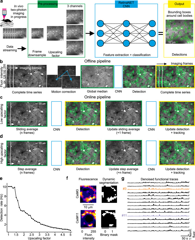
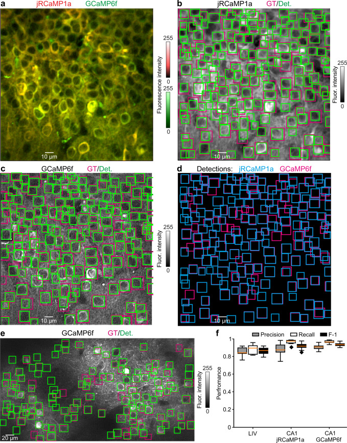
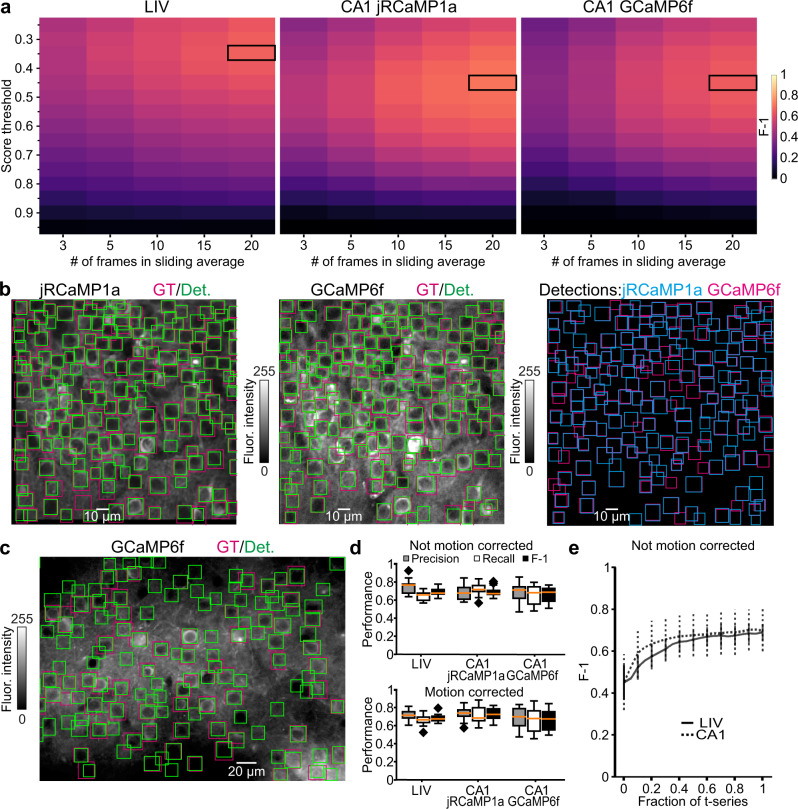
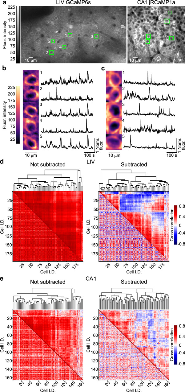
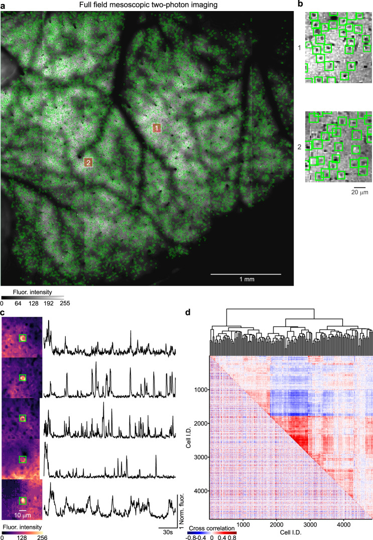
In vivo two-photon calcium imaging is a powerful approach in neuroscience. However, processing two-photon calcium imaging data is computationally intensive and time-consuming, making online frame-by-frame analysis challenging. This is especially true for large field-of-view (FOV) imaging. Here, we present CITE-On (Cell Identification and Trace Extraction Online), a convolutional neural network-based algorithm for fast automatic cell identification, segmentation, identity tracking, and trace extraction in two-photon calcium imaging data. CITE-On processes thousands of cells online, including during mesoscopic two-photon imaging, and extracts functional measurements from most neurons in the FOV. Applied to publicly available datasets, the offline version of CITE-On achieves performance similar to that of state-of-the-art methods for offline analysis. Moreover, CITE-On generalizes across calcium indicators, brain regions, and acquisition parameters in anesthetized and awake head-fixed mice. CITE-On represents a powerful tool to speed up image analysis and facilitate closed-loop approaches, for example in combined all-optical imaging and manipulation experiments.

Fig. 1. Structure and analysis pipeline of CITE-On.

a Schematic of the image detection process in CITE-On. During ongoing two-photon imaging acquisitions, individual frames are transferred to CITE-On as they are completed (left). A preprocessing step (green rectangle) is required ahead of image detection, including frame downsampling, image upscaling, and triplication of the upscaled image. The result of the preprocessing is then used as input to the CNN (blue rectangle). The CNN output is the detection of neuronal somata in the form of bounding boxes (green squares, greyscale image on the right). b CITE-On offline pipeline starts with the complete t-series and the correction of motion artifacts (blue arrow, motion correction). Frame downsampling is performed by computing the global median projection of the t-series. The upscaled and triplicated global median (green) is fed to the CNN (blue), a single detection is performed, and the bounding boxes (detection, green squares) are projected onto each frame of the complete t-series (yellow). The color scale shown on the left in this panel applies to all grayscale images in this figure. c In the online pipeline, for data requiring low upscaling factors, a sliding average projection of the first n frames of the ongoing t-series is calculated in the frame downsampling preprocessing step (green). This image is upscaled and triplicated, processed by the CNN (blue), producing the first detection (yellow). As the next frame of the t-series is acquired, a new sliding average is computed, again on n frames, but starting from the second frame of the acquisition and including the n + 1^th one (green). The CNN processes this image (blue), updating the detections and starting the tracking system (yellow). d For data requiring high upscaling factors, the pipeline is similar to that in c, but instead of a sliding average, a step average is calculated on n frames as the frame downsampling preprocessing step (green). Detections are updated every n new frames. e Detection rates as a function of the magnitude of the upscaling factor. The maximum detection rate is 10 Hz for upscaling factor between 1 and 1.5. f Representative average fluorescence of pixels inside the bounding box relative to two cells (cell #3 and cell #11), calculated in a single frame of the LIV dataset (GCaMP6s, pseudocolor, left). Associated dynamic segmentation mask in the same frame (binary mask, right). g Functional traces from N = 15 representative cells extracted with online CITE-On pipeline. Traces from cells displayed in f are shown in orange and purple.

Fig. 2. CITE-On offline cell detection performance.

a Representative fluorescence median projection showing jRCaMP1a (red) and GCaMP6f (green) expressing CA1 neurons. b Ground truth (GT, magenta) and CITE-On detections (Det, green) for the jRCaMP1a channel of the image shown in a. c Same as in (b), but for the GCaMP6f channel. d Superposition of CITE-On detections on jRCaMP1a (cyan) and GCaMP6f (magenta) channels. e Representative median projection from the LIV dataset with GT (magenta) and CITE-On detections (green). f Boxplots showing performance as Precision (gray), Recall (white), and F-1 score (black) obtained with the offline CITE-On pipeline on the validation t-series of the LIV (N = 13), CA1 jRCaMP1a (N = 12), and CA1 GCaMP6f (N = 12) datasets. The orange line in all boxplots indicates the median, the bounds of the boxes represent the 75th and 25th percentiles (i.e., the interquartile range (IQR)), and the whiskers correspond to the highest value or lowest value of the distribution. If the lowest or highest values are outliers (i.e., >1.5 *IQR from the bounds of the boxes) the whiskers correspond to 1.5 *IQR. Outliers are represented as black diamonds.

Fig. 3. CITE-On online cell detection performance.

a Best parameter search for frame downsampling: F-1 score (pseudocolor) as a function of score threshold (vertical axis) and number of frames in the sliding average (horizontal axis) for LIV (left), CA1 jRCaMP1a (middle), and CA1 GCaMP6f (right). The maximal F-1 is indicated with the black rectangle. b Fluorescence median projections of one representative FOV for CA1 jRCaMP1a (left) and one FOV for CA1 GCaMP6f (middle). GT (magenta) and online detections at the end of the t-series (Det, green) are also shown. In the rightmost panel, the online detections of jRCaMP1a (cyan) and GCaMP6f (magenta) at the end of the t-series are shown. c Same as in b but for a representative LIV t-series. d Top: boxplots showing online performance as Precision (gray), Recall (white), and F-1 (black) for all t-series in the validation datasets (LIV, N = 13; CA1 jRCaMP1a, N = 12; CA1 GCaMP6f, N = 12). No motion correction was performed. Bottom: same as top, but for the motion-corrected t-series. The orange line in all boxplots (in top and bottom panels) is the median, the bounds of the boxes are the 75th and 25th percentiles (i.e., the interquartile range (IQR)), and the whiskers correspond to the highest value or lowest value of the distribution. If the lowest or highest values are outliers (i.e., >1.5 *IQR from the bounds of the boxes), the whiskers correspond to 1.5 *IQR. Outliers are represented as black diamonds. Results of Kolmogorov–Smirnov test for performance in not motion-corrected t-series vs. motion-corrected t-series from LIV: p = 0.54 for F-1, p = 0.15 for Precision, p = 0.38 for Recall, N = 13 t-series. Results of two-sided Kolmogorov–Smirnov test for performance in not motion-corrected t-series vs. motion-corrected t-series from CA1 jRCaMP1a: p = 0.16 for F-1, p = 0.20 for Precision, p = 0.20 for Recall, N = 12 t-series. Results of Kolmogorov–Smirnov test for performance in not motion corrected vs. motion-corrected t-series from CA1 GCaMP6f: p = 0.18 for F-1, p = 0.28 for Precision, p = 0.22 for Recall, N = 12 t-series. e F-1 values as a function of the fraction of the total length of the t-series for not-motion corrected data (N = 13 t-series for LIV, N = 24 t-series for CA1, including N = 12 t-series for CA1 jRCaMP1a and N = 12 t-series for CA1 GCaMP6f t-series).

Fig. 4. Fast extraction of fluorescence traces using CITE-On.

a Fluorescence median projection showing representative FOVs from the LIV GCaMP6s (left) and the CA1 jRCaMP1a (right) datasets. True positive bounding boxes for five CITE-On identified cells in each FOV are shown in green. b Left: the five cells indicated in the LIV t-series displayed in a are shown at an expanded spatial scale. Right: fluorescence traces for the cells shown in the left panel were thresholded and background subtracted (see “Methods”). c Same as in b but for the CA1 t-series in a. d Lower-left triangle: cross-correlation matrix for all functional traces extracted from true positive detection in the LIV GCaMP6s t-series displayed in a. Upper-right triangle: corresponding dendrogram sorting. The left matrix shows signals before background subtraction. The right matrix after background subtraction. e Same as in d, but for the CA1 jRCaMP1a t-series shown in a.

Fig. 5. CITE-On offline cell detection performance on never-before-seen data.

a–e Best parameter search for frame upscaling factor: F-1 score (pseudocolor) as a function of upscaling factor and score threshold for the Allen Brain Observatory (ABO) ABO_sup (a), ABO_deep (b), and Neurofinder (NF) NF_train (c), NF_test (d) and VPM (e) datasets. The maximal F-1 is indicated by the black rectangle. The pseudocolor scale in (e) applies to a–d. f Optimized upscaling factor as a function of the ratio between the FOV area and the bounding box area for all acquisitions in the validation datasets. Each dot represents a single t-series (green, ABO_sup and ABO_deep together, N = 19; purple, NF_train, N = 19; red, NF_test, N = 9; brown, VPM, N = 9; orange, CA1 jRCaMP1a and GCaMP6f together, N = 24; gray, LIV, N = 13). The dotted line represents the linear fit of the data (R² = 0.942). g Boxplots showing performance as Precision (gray), Recall (white), and F-1 (black) for all t-series in the ABO_sup (N = 9), ABO_deep (N = 10), NF_train (N = 19), NF_test (N = 9), and VPM (N = 9) datasets. The orange line in all boxplots is the median, the bounds of the boxes are the 75th and 25th percentiles (i.e., the interquartile range (IQR)), and the whiskers correspond to the highest value or lowest value of the distribution. If the lowest or highest values are outliers (i.e., >1.5 *IQR from the bounds of the boxes) the whiskers correspond to 1.5 *IQR. Outliers are represented as black diamonds.

Fig. 6. CITE-On cell detection performance compared to state-of-the-art methods.

a, b Precision (left), Recall (middle), and F-1 score (right) in cell detection for CITE-On and other methods (for other methods plotted data are reported from ref. ). CITE-On performance is evaluated on ABO_sup (a, N = 9 t-series), ABO_deep (b, N = 10 t-series). CITE-On performance is calculated using our consensus ground truth (“ground truth from this work”, left of the vertical dotted line) or using the ground truth reported in Soltanian-Zadeh et al. (right of the vertical dotted line). CITE-On performance is shown in bloxplots, the performance of other methods is shown as mean ± s.d from ref. . The orange line in all boxplots is the median, the bounds of the boxes are the 75th and 25th percentiles (i.e., the interquartile range (IQR)), and the whiskers correspond to the highest value or lowest value of the distribution. If the lowest or highest values are outliers (i.e., >1.5 *IQR from the bounds of the boxes) the whiskers correspond to 1.5 *IQR. Outliers are represented as black diamonds.

Fig. 7. CITE-On data processing of never-before-seen recordings.

a Median projection of a representative t-series from the ABO dataset showing GCaMP6f expressing cortical neurons. CITE-On true positives (CITE-On, green) and true positives provided by the Allen Brain Observatory (ABO, magenta) are shown. b Same as in a with CITE-On true positives (green) and STNeuroNET true positives (magenta). c Superposition of CITE-On (green), ABO (magenta), and STNeuroNET (cyan) true positives. d Left: 24 representative cells detected by CITE-On and identified as true positives in ABO and STNeuroNET. The CITE-On-identified bounding box is represented in green. Right: corresponding CITE-On extracted fluorescence traces. e Same as in d for four representative CITE-On only cells. These fours cells were not included in the GT of the ABO dataset and of the STNeuroNET GT reported in the ref. , either as true or false positives. f Cross-correlation matrix for all functional traces extracted from true positive (TP) detections in the t-series displayed in a. Cell identities are grouped with hierarchical dendrogram sorting. The pseudocolor scale indicates the cross-correlation value.

Fig. 8. CITE-On online cell detection performance on never-before-seen datasets.

a–e Best parameter search for frame downsampling: F-1 score (pseudocolor) as a function of score threshold and number of frames for the ABO_sup (a), ABO_deep (b), NF_train (c), NF_test (d), and VPM (e) datasets. The maximal F-1 is indicated by the black rectangle. The pseudocolor scale in (e) applies to (a–d). For the ABO_sup, ABO_deep datasets the sliding average frame downsampling approach was used, while for the NF_test, NF_train, and VPM datasets, the step average approach was implemented. f–h Left: median projection of a representative t-series from the ABO_sup (f), NF_train (g), and VPM (h) datasets. GT (magenta) and online CITE-On detections (green bounding boxes) are shown. Right: bounding boxes (yellow) corresponding to true positives (TP) are shown. The greyscale in h applies also to f, g. i Boxplots showing online detection performance of Precision (gray), Recall (white), and F-1 (black) for all t-series in the ABO_sup (N = 9), ABO_deep (N = 10), NF_train (N = 19), NF_test (N = 9), and VPM (N = 9) datasets. The orange line in all boxplots is the median, the bounds of the boxes are the 75th and 25th percentiles (i.e., the interquartile range (IQR)), and the whiskers correspond to the highest value or lowest value of the distribution. If the lowest or highest values are outliers (i.e., >1.5 *IQR from the bounds of the boxes) the whiskers correspond to 1.5 *IQR. Outliers are represented as black diamonds. j F-1 values as a function of the fraction of processed t-series for ABO (green, N = 19 t-series), NF_test (red, N = 9 t-series), NF_train (purple, N = 19 t-series), and VPM (brown, N = 9 t-series) datasets. Ten frames sliding averages for ABO; detection rate, 5 Hz. Step median of 20 frames and 200 frames for VPM and NF datasets; detection rate, 0.3 Hz and 0.035 Hz for VPM and NF datasets, respectively.

Fig. 9. CITE-On analysis of mesoscopic two-photon imaging t-series.

a, b Median projection of a mesoscopic imaging t-series showing GCaMP6s expressing neurons (mesoscopic data from ref. ). Green boxes indicate cells detected by CITE-On (total: 4842 cells). Two regions are highlighted by the red and white squares, and are shown at an expanded spatial scale in b. Greyscale in a applies also to b. c Left: five representative cells detected by CITE-On. The brightest cell in each FOV was selected. Right: corresponding CITE-On extracted fluorescence traces in the first 230 s of the t-series. d Cross-correlation matrix (bottom-left triangle) calculated on the background-subtracted traces extracted by CITE-On on all detected cells in the first 7000 frames and relative dendrogram (top-right triangle).

References

1. Helmchen F, Denk W. Deep tissue two-photon microscopy. Nat. Methods. 2005;2:932–940. - PubMed
1. Wang T, et al. Three-photon imaging of mouse brain structure and function through the intact skull. Nat. Methods. 2018;15:789–792. - PMC - PubMed
1. Chen TW, et al. Ultrasensitive fluorescent proteins for imaging neuronal activity. Nature. 2013;499:295–300. - PMC - PubMed
1. Dana H, et al. Sensitive red protein calcium indicators for imaging neural activity. Elife. 2016;5:12727. - PMC - PubMed
1. Svoboda K, Yasuda R. Principles of two-photon excitation microscopy and its applications to neuroscience. Neuron. 2006;50:823–839. - PubMed
Publication types