. 2022 Mar 29;119(13):e2115699119.
doi: 10.1073/pnas.2115699119. Epub 2022 Mar 23.

Prediction-error neurons in circuits with multiple neuron types: Formation, refinement, and functional implications

Affiliations

Prediction-error neurons in circuits with multiple neuron types: Formation, refinement, and functional implications

Loreen Hertäg et al. Proc Natl Acad Sci U S A. .

Abstract

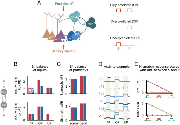
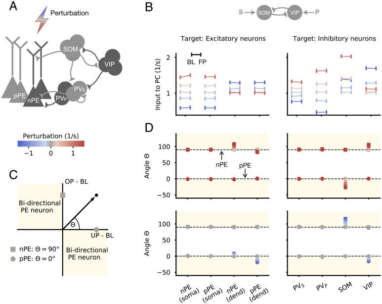
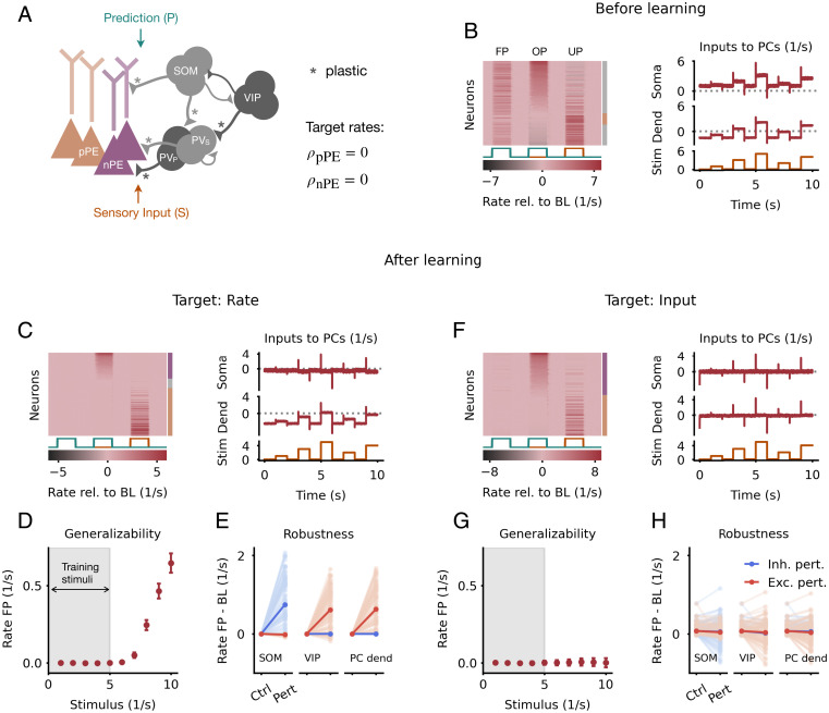
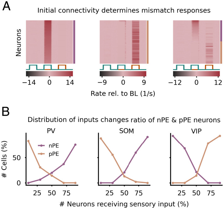
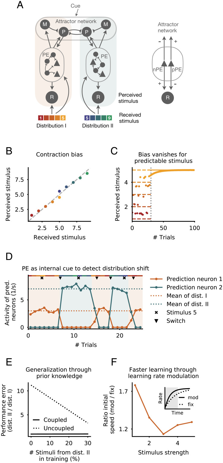
SignificanceAn influential idea in neuroscience is that neural circuits do not only passively process sensory information but rather actively compare them with predictions thereof. A core element of this comparison is prediction-error neurons, the activity of which only changes upon mismatches between actual and predicted sensory stimuli. While it has been shown that these prediction-error neurons come in different variants, it is largely unresolved how they are simultaneously formed and shaped by highly interconnected neural networks. By using a computational model, we study the circuit-level mechanisms that give rise to different variants of prediction-error neurons. Our results shed light on the formation, refinement, and robustness of prediction-error circuits, an important step toward a better understanding of predictive processing.

Keywords: homeostatic plasticity; inhibitory interneurons; prediction-error neurons; predictive processing; sensory coding.


Conflict of interest statement

The authors declare no competing interest.

Figures

Fig. 1.
Fig. 1.
Multipathway E/I balance in nPE and pPE neurons. (A, Left) Network model with excitatory PCs and inhibitory PV, SOM, and VIP neurons. Connections from PCs are not shown for the sake of clarity. In a PE circuit, PCs act as either nPE or pPE neurons. The somatic compartment of PCs and half of the PV neurons (PVS) receive the actual sensory input, while the dendritic compartment of PCs and the remaining PV neurons (PVP) receive the predicted sensory input. SOM and VIP neurons receive either actual or predicted sensory input. (A, Right) Sensory stimuli can be FP, OP, or UP. (B–E) Mean-field network derived from A with the SOM neuron receiving the actual sensory input and the VIP neuron receiving the predicted sensory stimulus. (B) In a PE circuit, the excitatory (red) and inhibitory (blue) inputs are balanced for FP sensory stimuli for both nPE and pPE neurons. This balance is preserved for UP stimuli (nPE neurons; Upper) or OP stimuli (pPE neurons; Lower). Stimulus strength is 1s1. Shown are the inputs without the excitatory background input that defines the BL firing rate. (C) Both nPE (Upper) and pPE (Lower) neurons exhibit balanced pathways onto both soma and dendrites. (D) Example activity of all neuron types for FP as well as OP and UP stimuli for a network parameterized to establish an E/I balance in the pathways. The vertical black bar denotes 3s1; the horizontal black bar denotes 500 ms. (E) Mismatch responses for nPE (Upper) and pPE (Lower) neurons scale with the difference between actual and predicted sensory inputs.
Fig. 2.
Fig. 2.
PE neurons are robust to moderate network perturbations. (A) Each neuron type/compartment of a mean-field network with nPE and pPE neurons is perturbed with an additional inhibitory or excitatory input. The same circuit as in Fig. 1 B–E is shown. SOM neurons receive the actual sensory input, while VIP neurons receive a prediction thereof. (B) Total input into PE neurons during the absence of sensory stimuli (BL) and for FP sensory stimuli (FP) for different perturbation strengths and different perturbation targets (Left shows compartments of PCs, and Right shows inhibitory neurons). Total inputs in both phases are almost equal as a result of the established E/I balance. Gray indicates no perturbation. (C) Illustration of nPE (square) and pPE (circle) neurons in the input space. Input space is defined by the total input to PCs for OP and UP sensory stimuli. nPE neurons lie on the positive part of the y axis, while pPE neurons lie on the positive part of the x axis. Beige areas denote bidirectional PE neurons. Θ defines the angle in the input space. (D) Θ for different perturbation strengths (Upper: excitatory; Lower: inhibitory) and different perturbation targets (Left: compartments of PCs; Right: inhibitory neurons). Perturbations have minor effects on nPE and pPE neurons, especially when BL firing rates of PCs are low.
Fig. 3.
Fig. 3.
nPE and pPE neurons develop through inhibitory plasticity with a low homeostatic target rate. (A) Heterogeneous network model with excitatory PCs and inhibitory PV, SOM, and VIP neurons. All PCs receive actual sensory input at the somatic compartment and a prediction thereof at the dendritic compartment; 50% of the PV neurons, 70% of the SOM neurons, and 30% of the VIP neurons receive the sensory stimuli. The remaining cells receive the prediction. Connections marked with an asterisk undergo experience-dependent plasticity. Target rates for PCs are set to zero. (B) Responses of and inputs to PCs before learning. (B, Left) Responses relative to BL of all PCs for FP, OP, and UP stimuli sorted by amplitude of mismatch response in OP. Almost none of the PCs are classified as PE neurons summarized by the bar to the right (gray: no PE neuron; purple: nPE neuron; orange: pPE neuron). (B, Right) Mean input into both soma and dendrites of PCs for FP stimuli. Inputs are not balanced. (C) Same as in B but after learning with an inhibitory plasticity rule that establishes a zero target rate in PCs. (C, Left) Most of the PCs are either nPE (purple) or pPE (orange) neurons (indicated by the colored bar to the right). (C, Right) Mean inputs into both soma and dendrites of PCs for FP stimuli are not balanced. (D) Median and SEM of PC responses for FP sensory stimuli. The gray area indicates the range of stimuli used during learning. Sensory stimuli that are larger than the training stimuli evoke neuron responses. (E) Inhibitory (blue) and excitatory (red) perturbations can cause the PE neurons to deviate from their BL activity. Light colors denote single neurons, and dark colors denote the population average. (F–H) Same as C–E but with an inhibitory plasticity rule that establishes a target for the total input to PCs (target: zero). (F, Left) Most of the PCs are either nPE (purple) or pPE (orange) neurons (indicated by the colored bar to the right). (F, Right) Mean inputs into both soma and dendrites of PCs for FP stimuli are balanced. (G) Sensory stimuli that are larger than the training stimuli evoke only minor neuron responses. The PE neurons can generalize beyond the training stimuli. (H) PE neurons are robust to inhibitory and excitatory perturbations after learning. Ctrl, control; Pert, perturbation.
Fig. 4.
Fig. 4.
Initial connectivity and distribution of inputs onto interneurons determine mismatch responses of PE neurons. (A) For three different initial weight configurations, the network forms nPE neurons (Left), pPE neurons (Center), or both (Right). Mean initial weights: (1+wPP)/wEP=0.6,wPS=0.75, and wPV=2 (Left); (1+wPP)/wEP=0.4,wPS=2, and wPV=0.75 (Center); (1+wPP)/wEP=0.4,wPS=1.75, and wPV=1.25 (Right). SOM neurons and 50% of the PV neurons receive the actual sensory input, while VIP neurons and the remaining PV neurons receive a prediction thereof. wEP, weight from PV neurons onto soma of PCs; wPP, recurrent inhibition between PV neurons; wPS, weight from SOM neurons onto PV neurons; wPV, weight from VIP neurons onto PV neurons. (B) The number of PV neurons (Left), SOM neurons (Center), or VIP neurons (Right) that receive the actual sensory input is varied. The ratio of nPE and pPE neurons changes with the distribution of actual and predicted sensory inputs onto the interneurons. For the neuron types for which the distribution of inputs was not varied, the fraction of neurons receiving the actual sensory input was set to 0.5.
Fig. 5.
Fig. 5.
The role of PE neurons in biased perception. (A, Left) Attractor–memory network with PE neurons. The network consists of two subnetworks, the neurons of which are only responsive to a subset of stimuli. Each subnetwork comprises a representation neuron (R) and a PE circuit. Both R and PE neurons receive sensory stimuli of either of two uniform distributions. The PE circuit is connected to both the R and an attractor network that comprises memory neurons (M) and prediction neurons (P). The two prediction neurons are mutually connected via inhibitory synapses and receive excitatory input from the memory neuron of their respective subnetwork. (A, Right) nPE and pPE neurons connect to M, P, and R neurons with opposing sign. (B) The PE neurons establish a contraction bias for both distributions. A stimulus that is smaller than the distribution mean is perceived stronger, while a stimulus that is larger than the distribution mean is perceived weaker. (C) The response of the representation neuron becomes unbiased after the transition (dotted vertical line) from a uniform distribution to a binary distribution because the stimulus becomes predictable. (D) The network does not receive a cue signal indicating the distribution from which the stimuli are drawn. After an uncued switch from one distribution to another, the former inactive prediction neuron becomes active, and the former active prediction neuron becomes inactive (network switching is denoted by a triangle). This is the result of the PE neurons and the mutual inhibition between both prediction neurons. Stimulus present in both distributions does not evoke a switch (denoted by x). Shaded areas denote the distributions from which the stimuli are drawn. (E) Both distributions equally change from uniform to binary (to maximal values of former uniform distributions). A network in which the PE neurons are equally coupled to both memory neurons (solid line) shows the same performance error for both distributions independent of the training set composition. A network in which the PE neurons are only coupled to the memory neuron of their respective subnetwork (dashed line) shows a larger error for the distribution that is underrepresented during training. (F) Speed of learning (defined as the averaged change of activity in the first 50 ms; the gray area in Inset) is increased when PE neuron activity modulates the learning rate based on the degree of the stimulus’ unpredictability compared with a fixed learning rate (solid vs. dashed lines in Inset).

Similar articles

Cited by

References

    1. Rao R. P., Ballard D. H., Predictive coding in the visual cortex: A functional interpretation of some extra-classical receptive-field effects. Nat. Neurosci. 2, 79–87 (1999). - PubMed
    1. Friston K., A theory of cortical responses. Philos. Trans. R. Soc. Lond. B Biol. Sci. 360, 815–836 (2005). - PMC - PubMed
    1. Keller G. B., Mrsic-Flogel T. D., Predictive processing: A canonical cortical computation. Neuron 100, 424–435 (2018). - PMC - PubMed
    1. Schultz W., Dickinson A., Neuronal coding of prediction errors. Annu. Rev. Neurosci. 23, 473–500 (2000). - PubMed
    1. Keller G. B., Bonhoeffer T., Hübener M., Sensorimotor mismatch signals in primary visual cortex of the behaving mouse. Neuron 74, 809–815 (2012). - PubMed

MeSH terms

LinkOut - more resources