. 2022 Mar 22;38(12):110547.
doi: 10.1016/j.celrep.2022.110547.

A 3D transcriptomics atlas of the mouse nose sheds light on the anatomical logic of smell

Affiliations

A 3D transcriptomics atlas of the mouse nose sheds light on the anatomical logic of smell

Mayra L Ruiz Tejada Segura et al. Cell Rep. .

Abstract

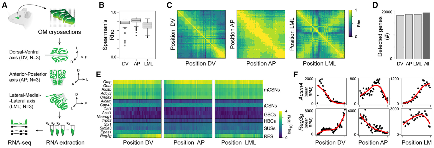
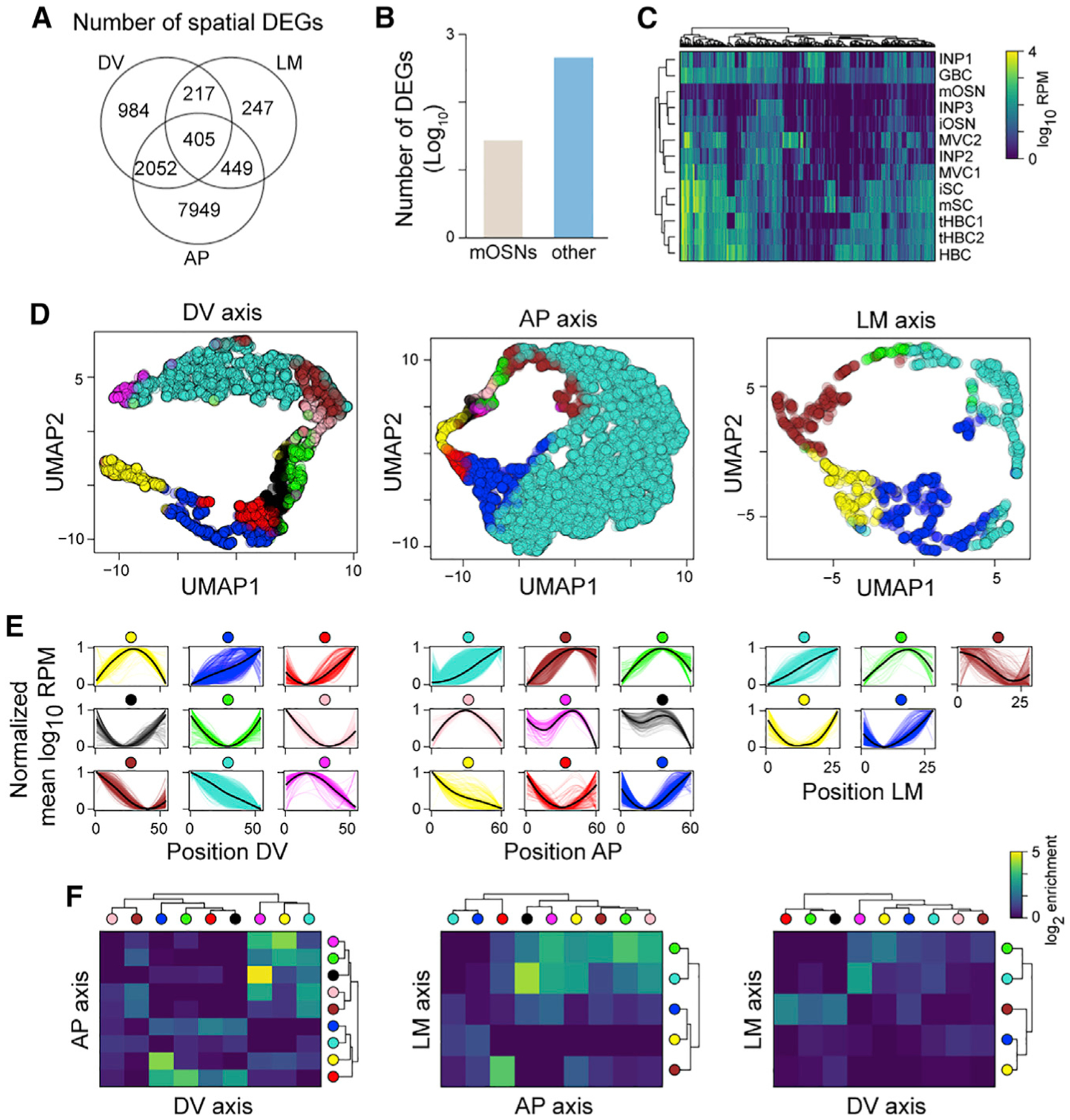
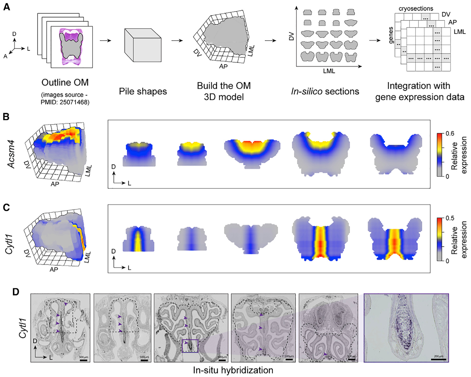
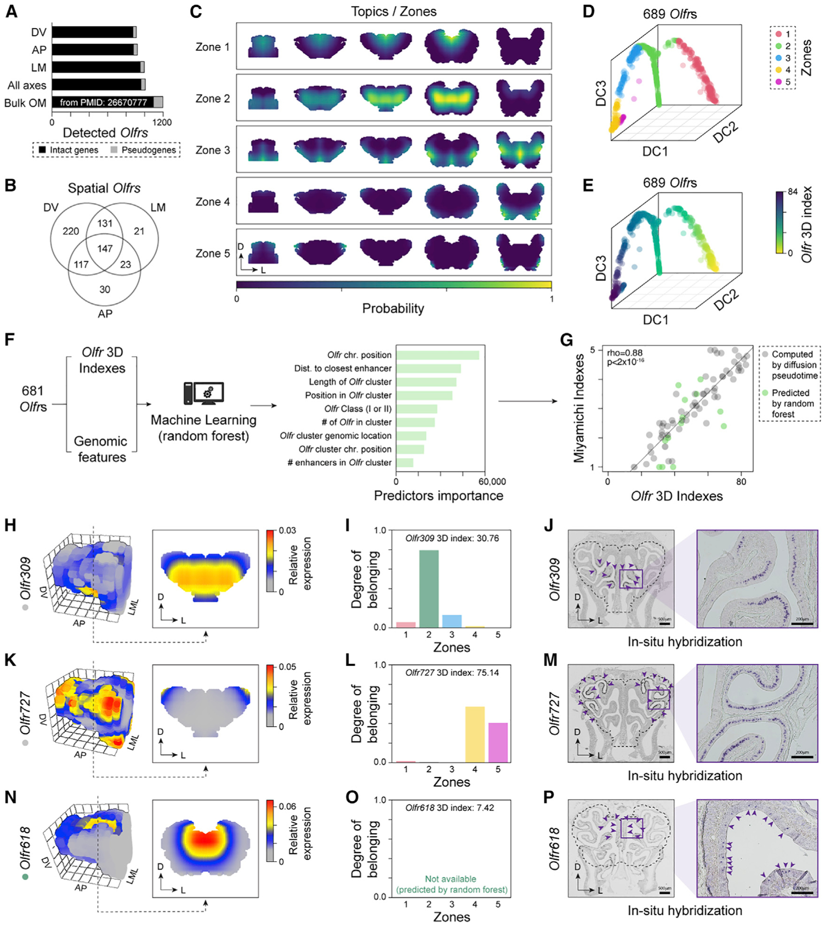
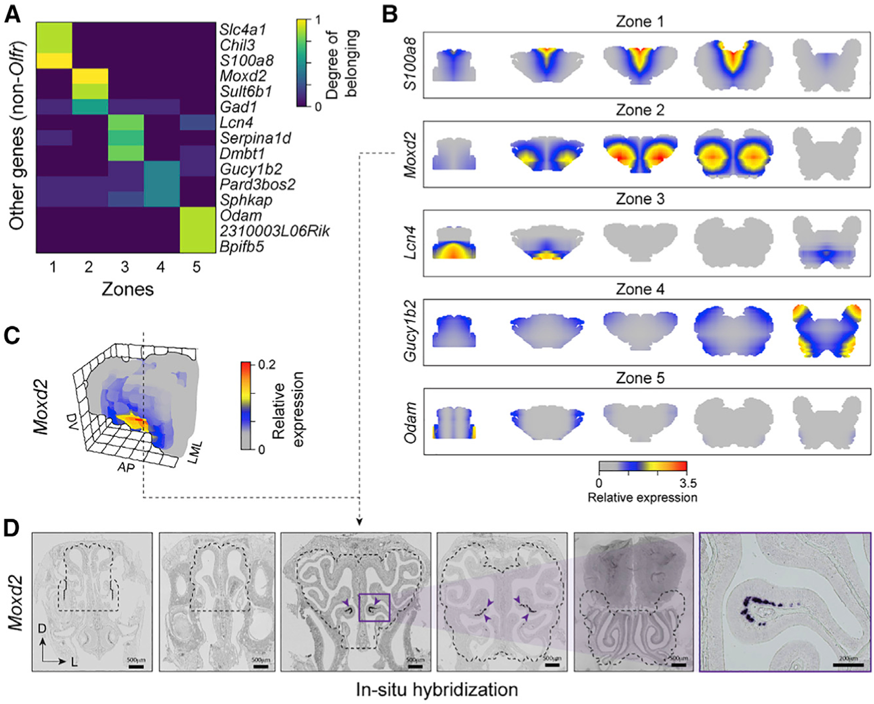
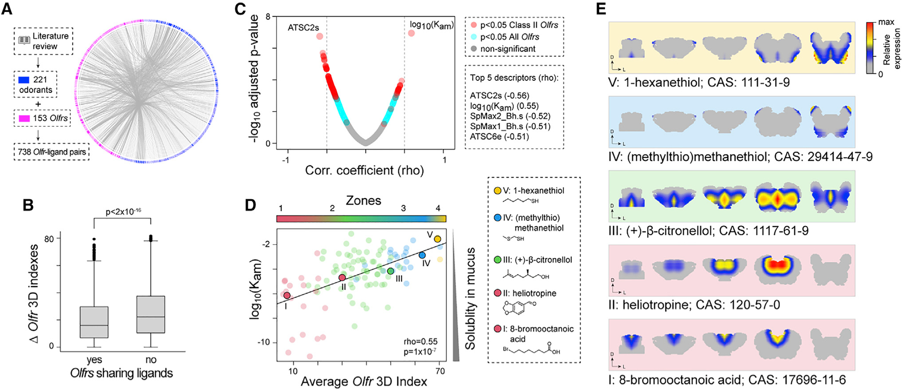
The sense of smell helps us navigate the environment, but its molecular architecture and underlying logic remain understudied. The spatial location of odorant receptor genes (Olfrs) in the nose is thought to be independent of the structural diversity of the odorants they detect. Using spatial transcriptomics, we create a genome-wide 3D atlas of the mouse olfactory mucosa (OM). Topographic maps of genes differentially expressed in space reveal that both Olfrs and non-Olfrs are distributed in a continuous and overlapping fashion over at least five broad zones in the OM. The spatial locations of Olfrs correlate with the mucus solubility of the odorants they recognize, providing direct evidence for the chromatographic theory of olfaction. This resource resolves the molecular architecture of the mouse OM and will inform future studies on mechanisms underlying Olfr gene choice, axonal pathfinding, patterning of the nervous system, and basic logic for the peripheral representation of smell.

Keywords: CP: Neuroscience; RNA-seq; machine learning; odorant; olfaction; olfactory epithelium; olfactory mucosa; spatial transcriptomics.


Conflict of interest statement

Declaration of interests The authors declare no competing interests.

Figures

Figure 1.
Figure 1.. Application of TOMO-seq to mouse OM
(A) Experimental design. TOMO-seq was performed on nine tissue samples, from which three were sliced along the dorsal-ventral axis (DV), three along the anterior-posterior axis (AP), and three along the lateral-medial-lateral axis (LML). (B) Boxplots showing the distributions of Spearman’s correlation coefficients (rho) between replicates in each axis. (C) Heatmaps showing Spearman’s correlation between gene expression patterns at different positions along the three axes. (D) Number of detected genes along each axis separately or across the whole dataset. Genes were considered as detected when they had at least one normalized count in at least 10% of the samples from one axis. (E) Heatmaps of log10 normalized expression (after combining the three replicates per axis) of OM canonical markers along the three axes (GBCs, globose basal cells; HBCs, horizontal basal cells; iOSNs, immature olfactory sensory neurons; mOSNs, mature olfactory sensory neurons; RESs, respiratory epithelium cells; RPM, reads per million; SUSs, sustentacular cells). (F) Normalized expression of canonical OM spatial marker genes along the three axes. Red line shows fits with local polynomial models.
Figure 2.
Figure 2.. Genes with non-random spatial patterns across different cell types in the OM
(A) Venn diagram showing the numbers of spatial differentially expressed genes (DEGs) along each axis. (B) Bar plot showing the log10 number of spatial DEGs that are mOSN specific (“mOSNs”) or that are detected only in cell types other than mOSNs (“other”). (C) Heatmap of log10 mean expression per cell type of genes that are not expressed in mOSNs but only in other OM cell types (INPs, immediate neuronal precursors; iSCs, immature sustentacular cells; mSCs, mature sustentacular cells; MVCs, microvillous cells; mSCs, mature sustentacular cells). (D) UMAP plots of spatial DEGs along the three axes (n = 3 per axis). Each gene is colored according to the cluster it belongs to. (E) Normalized average expression patterns of spatial DEGs clusters along the three axes. (F) Heatmap showing the log2 enrichment over the random case for the intersection between lists of genes belonging to different clusters (indicated by colored circles) across pairs of axes.
Figure 3.
Figure 3.. The 3D reconstruction of the OM
(A) Schematic of 3D shape reconstruction strategy. Images of 2D slices along the AP axis of the OM were piled together to build an in silico 3D model of OM, which can also be used to visualize in silico sections. This 3D model, together with the gene expression data along each axis, was the input of the iterative proportional fitting algorithm, which allowed us to estimate a 3D expression pattern for any gene. (B and C) Reconstruction of the 3D expression patterns of the Acsm4 (B) and Cytl1 (C) in the OM, visualized in 3D and in OM coronal sections taken along the AP axis. (D) ISH experiment validating Cytl1 spatial expression pattern reconstructed in (C); note that Cytl1 is expressed in the septal region all along the OM. Purple arrowheads indicate the location of labeled cells. The dotted outline marks the borders of the OM dissected and used in the RNA-seq experiments and for the construction of the 3D model.
Figure 4.
Figure 4.. Zonal organization of Olfrs in the OM
(A) Number of Olfrs detected in our data and in an OM bulk RNA-seq data (Saraiva et al., 2015b). (B) Venn diagram of spatially differentially expressed Olfrs per axis (n = 3 per axis). (C) Visualization of the five zones across the OM (coronal sections) estimated with a latent Dirichlet allocation algorithm. The colors indicate the probability (scaled by its maximum value) that a position belongs to a given zone. (D) Diffusion map of Olfrs. Genes are colored based on the zone they fit in the most. DC, diffusion component. (E) Same as (D), with Olfrs colored by their 3D index. (F) We fitted a random forest algorithm to the 3D indices of 681 spatial Olfrs using nine genomic features as predictors. After training, the random forest was used to predict the 3D indices of 697 Olfrs that have too low levels in our data. (G) 3D indices versus the indices of 80 Olfrs estimated in Miyamichi et al. (2005) from ISH data. Black circles indicate Olfrs detected in our dataset; green circles are Olfrs whose indices were predicted with random forest. The correlation coefficients computed separately on these two sets of Olfrs are, respectively, rho = 0.92 (p < 2 × 10⁻¹⁶) and rho = 0.69 (p = 0.009). (H–P) Predicted expression patterns (H, K, and N), degrees of belonging (I, L, and O), and ISH (J, M, and P) for Olfr309, Olfr727, and Olfr618, respectively. Purple arrowheads indicate the location of labeled cells. The dotted outline marks the borders of the OM dissected and used in the RNA-seq experiments and for the construction of the 3D model.
Figure 5.
Figure 5.. Zonal organization of non-Olfr genes in the OM
(A) Heatmap of degrees of belonging of most zone-specific non-Olfr genes. (B) 3D gene expression pattern (coronal sections) of most topic-specific non-Olfrs for each topic along the AP axis. (C) Reconstruction of the 3D expression pattern of the gene Moxd2 in the OM. (D) ISH experiment validating Moxd2 spatial expression pattern reconstructed in (B) and (C). Purple arrowheads indicate the location of ISH-labeled cells. The dotted outline marks the borders of the OM dissected and used in the RNA-seq experiments and for the construction of the 3D model.
Figure 6.
Figure 6.. Physiological role of the zones
(A) Circular network illustrating the pairs of Olfrs and ligands that we found in the literature. (B) Boxplots showing the distributions of the absolute value of 3D index differences between pairs of Olfrs sharing at least one ligand versus pairs of Olfrs without cognate ligands in common. The difference between the two distributions is statistically significant (p < 2 × 10⁻¹⁶; Wilcoxon rank-sum test). (C) Scatterplot showing the Spearman correlation coefficients between the ligands’ mean 3D indices and molecular descriptors and the corresponding −log10(adjusted p value). Turquoise circles indicate the descriptors having a significant correlation only when both class I and II Olfrs are considered; red circles mark the descriptors with a significant correlation also when class I Olfrs are removed. (D) Scatterplot illustrating the correlation between air/mucus partition coefficients of the odorants and the average 3D indices of their cognate Olfrs. Only odorants for which we know at least two cognate Olfrs (110) were used here. Odorants are colored according to the zone they belong to (defined as the zone with the highest average degree of belonging computed over all cognate receptors). The five odorants highlighted in the plot by larger circles are indicated on the right-hand side, along with their molecular structure and common name. (E) Average expression pattern of the cognate Olfrs recognizing each of the five odorants highlighted in (D), including their respective CAS numbers.

Similar articles

Cited by

References

    1. Abaffy T, and Defazio AR (2011). The location of olfactory receptors within olfactory epithelium is independent of odorant volatility and solubility. BMC Res. Notes 4, 137. - PMC - PubMed
    1. Abaffy T, Matsunami H, and Luetje CW (2006). Functional analysis of a mammalian odorant receptor subfamily. J. Neurochem 97, 1506–1518. - PMC - PubMed
    1. Achim K, Pettit J-B, Saraiva LR, Gavriouchkina D, Larsson T, Arendt D, and Marioni JC (2015). High-throughput spatial mapping of single-cell RNA-seq data to tissue of origin. Nat. Biotechnol 33, 503–509. - PubMed
    1. Adipietro KA, Mainland JD, and Matsunami H (2012). Functional evolution of mammalian odorant receptors. PLoS Genet. 8, e1002821. - PMC - PubMed
    1. Aldinucci M, Bagnasco S, Lusso S, Pasteris P, Rabellino S, and Vallero S (2017). OCCAM: a flexible, multi-purpose and extendable HPC cluster. J. Phys. Conf. Ser 898, 082039.

Publication types

Substances

LinkOut - more resources