

Numerical Investigations of Urban Pollutant Dispersion and Building Intake Fraction with Various 3D Building Configurations and Tree Plantings
- PMID: 35329210
- PMCID: PMC8951778
- DOI: 10.3390/ijerph19063524
Numerical Investigations of Urban Pollutant Dispersion and Building Intake Fraction with Various 3D Building Configurations and Tree Plantings
Abstract
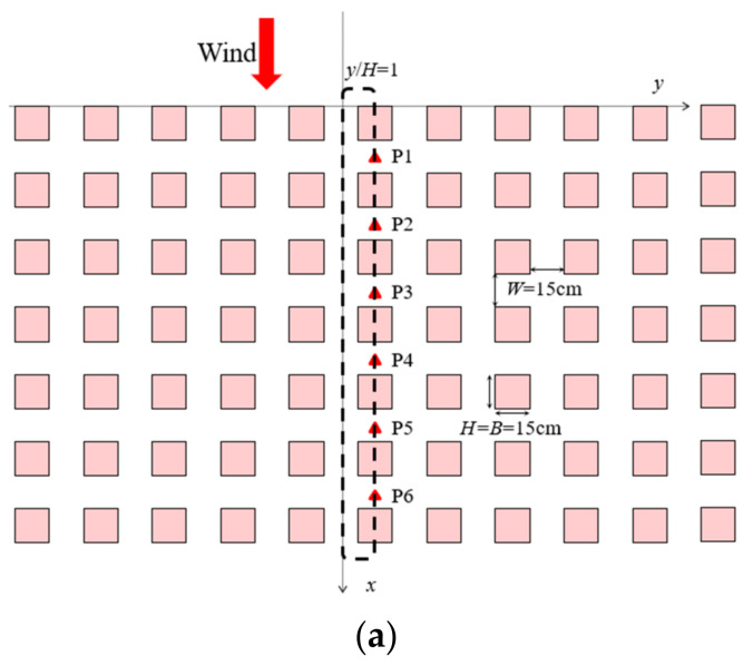
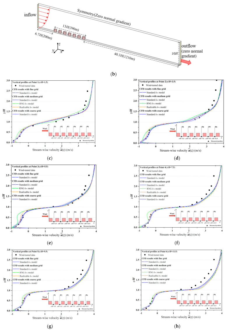
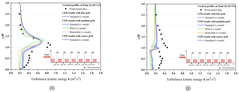
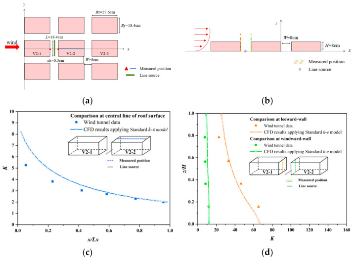
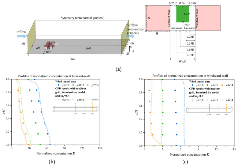
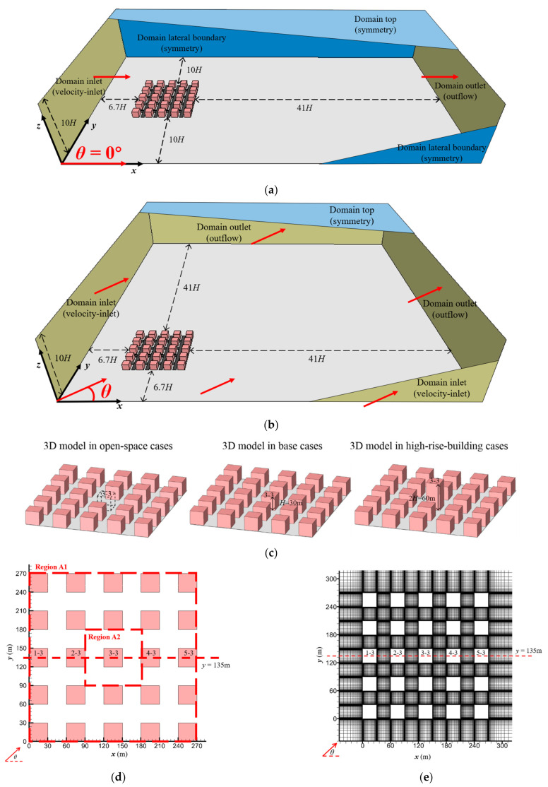
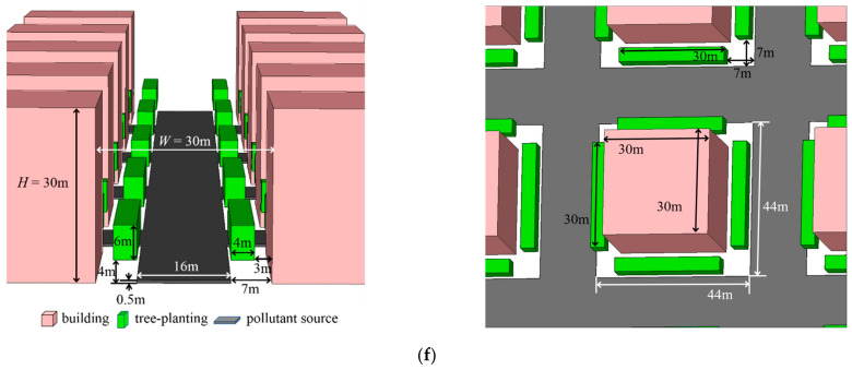
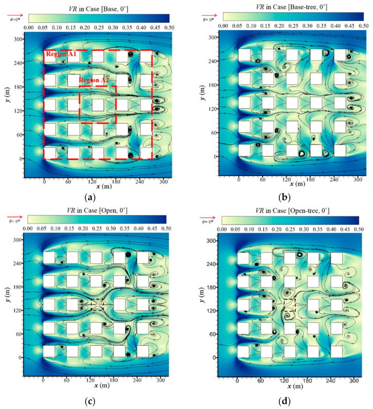
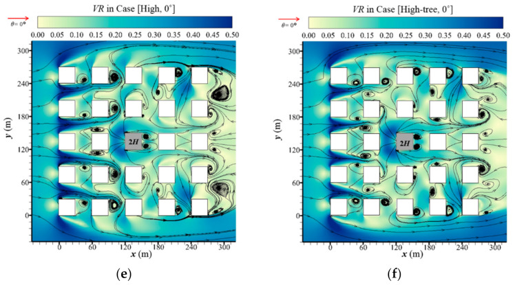
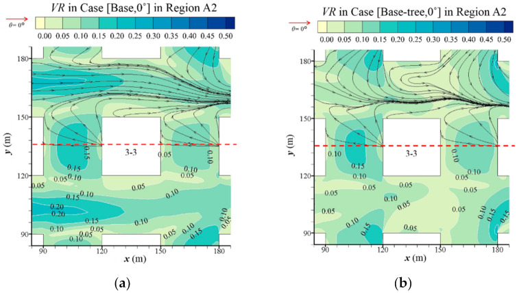
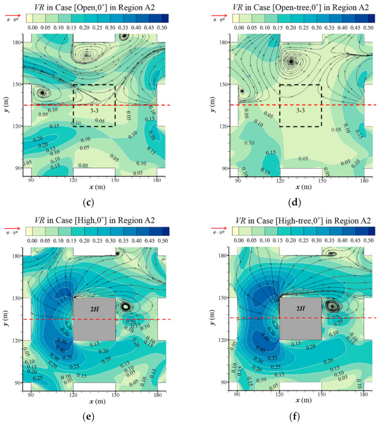
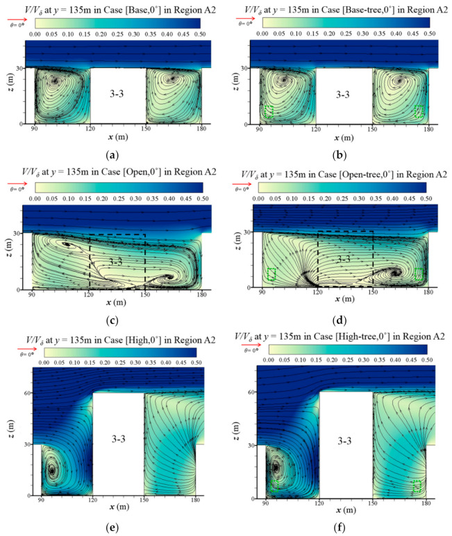
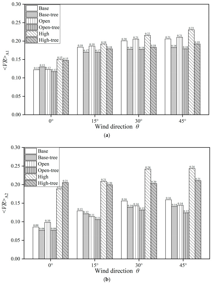
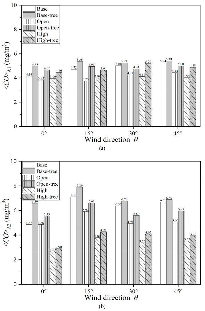
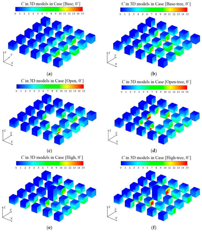
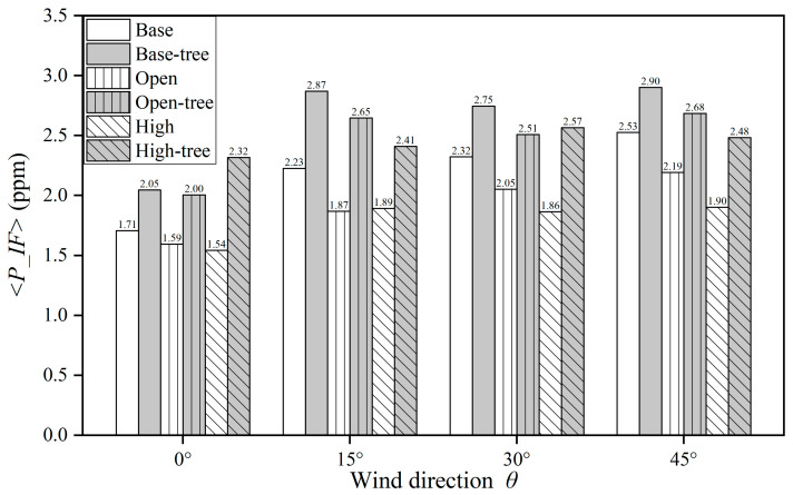
Rapid urbanisation and rising vehicular emissions aggravate urban air pollution. Outdoor pollutants could diffuse indoors through infiltration or ventilation, leading to residents’ exposure. This study performed CFD simulations with a standard k-ε model to investigate the impacts of building configurations and tree planting on airflows, pollutant (CO) dispersion, and personal exposure in 3D urban micro-environments (aspect ratio = H/W = 30 m, building packing density λp = λf = 0.25) under neutral atmospheric conditions. The numerical models are well validated by wind tunnel data. The impacts of open space, central high-rise building and tree planting (leaf area density LAD= 1 m2/m3) with four approaching wind directions (parallel 0° and non-parallel 15°, 30°, 45°) are explored. Building intake fraction <P_IF> is adopted for exposure assessment. The change rates of <P_IF> demonstrate the impacts of different urban layouts on the traffic exhaust exposure on residents. The results show that open space increases the spatially-averaged velocity ratio (VR) for the whole area by 0.40−2.27%. Central high-rise building (2H) can increase wind speed by 4.73−23.36% and decrease the CO concentration by 4.39−23.00%. Central open space and high-rise building decrease <P_IF> under all four wind directions, by 6.56−16.08% and 9.59−24.70%, respectively. Tree planting reduces wind speed in all cases, raising <P_IF> by 14.89−50.19%. This work could provide helpful scientific references for public health and sustainable urban planning.
Keywords: CFD simulation; open space; personal intake fraction; pollutant dispersion; urban tree planting; ventilation.
Conflict of interest statement
The authors declare no conflict of interest.
Figures
Similar articles
-
Influencing Factors on Airflow and Pollutant Dispersion around Buildings under the Combined Effect of Wind and Buoyancy-A Review.Int J Environ Res Public Health. 2022 Oct 8;19(19):12895. doi: 10.3390/ijerph191912895. Int J Environ Res Public Health. 2022. PMID: 36232193 Free PMC article. Review.
-
The impact of urban open space and 'lift-up' building design on building intake fraction and daily pollutant exposure in idealized urban models.Sci Total Environ. 2018 Aug 15;633:1314-1328. doi: 10.1016/j.scitotenv.2018.03.194. Epub 2018 Apr 2. Sci Total Environ. 2018. PMID: 29758884
-
Numerical simulation of the influence of building-tree arrangements on wind velocity and PM2.5 dispersion in urban communities.Sci Rep. 2022 Sep 30;12(1):16378. doi: 10.1038/s41598-022-20455-6. Sci Rep. 2022. PMID: 36180533 Free PMC article.
-
Aerodynamic effects of trees on pollutant concentration in street canyons.Sci Total Environ. 2009 Sep 15;407(19):5247-56. doi: 10.1016/j.scitotenv.2009.06.016. Epub 2009 Jul 10. Sci Total Environ. 2009. PMID: 19596394
-
Urban greenery for air pollution control: a meta-analysis of current practice, progress, and challenges.Environ Monit Assess. 2022 Mar 1;194(3):235. doi: 10.1007/s10661-022-09808-w. Environ Monit Assess. 2022. PMID: 35233683 Free PMC article. Review.
Cited by
-
Numerical analysis on the airflow organization of a blowing suction dust collector.Sci Rep. 2025 Mar 25;15(1):10244. doi: 10.1038/s41598-025-94767-8. Sci Rep. 2025. PMID: 40133433 Free PMC article.
-
Influencing Factors on Airflow and Pollutant Dispersion around Buildings under the Combined Effect of Wind and Buoyancy-A Review.Int J Environ Res Public Health. 2022 Oct 8;19(19):12895. doi: 10.3390/ijerph191912895. Int J Environ Res Public Health. 2022. PMID: 36232193 Free PMC article. Review.
-
Verification of the Perception of the Local Community concerning Air Quality Using ADMS-Roads Modeling.Int J Environ Res Public Health. 2022 Sep 1;19(17):10908. doi: 10.3390/ijerph191710908. Int J Environ Res Public Health. 2022. PMID: 36078624 Free PMC article.
References
Publication types
MeSH terms
Substances
LinkOut - more resources
Full Text Sources
Medical
Miscellaneous
