. 2022 Apr 11;62(7):1691-1711.
doi: 10.1021/acs.jcim.2c00044. Epub 2022 Mar 30.

GROMACS in the Cloud: A Global Supercomputer to Speed Up Alchemical Drug Design

Affiliations

GROMACS in the Cloud: A Global Supercomputer to Speed Up Alchemical Drug Design

Carsten Kutzner et al. J Chem Inf Model. .

Abstract

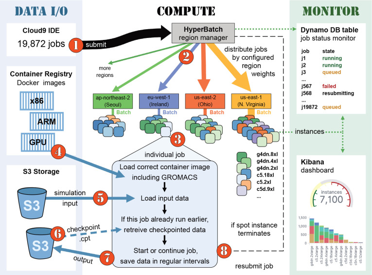
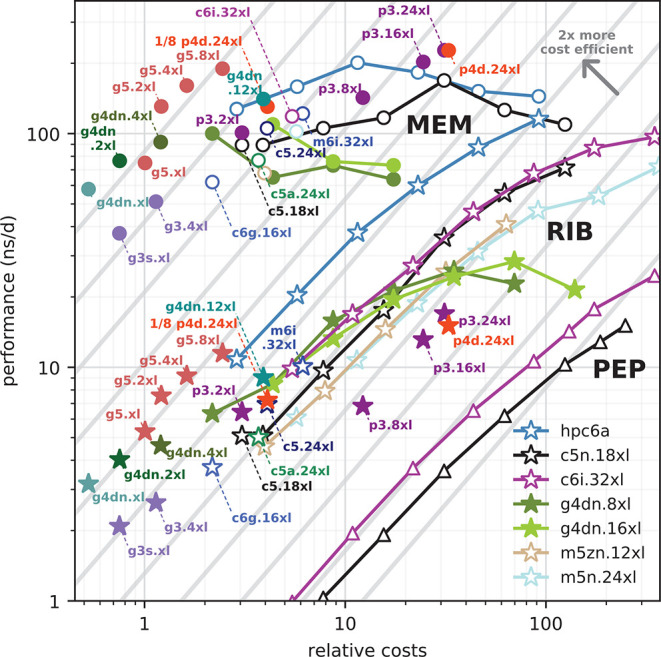
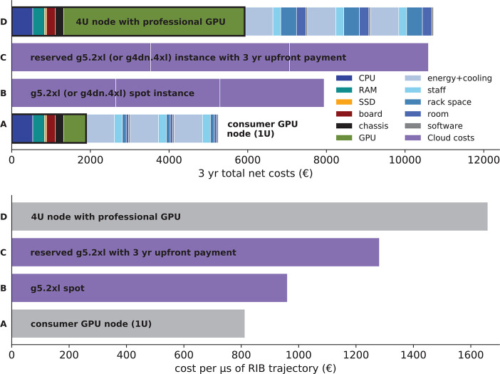
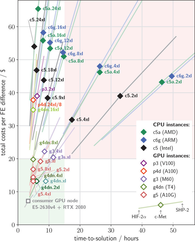
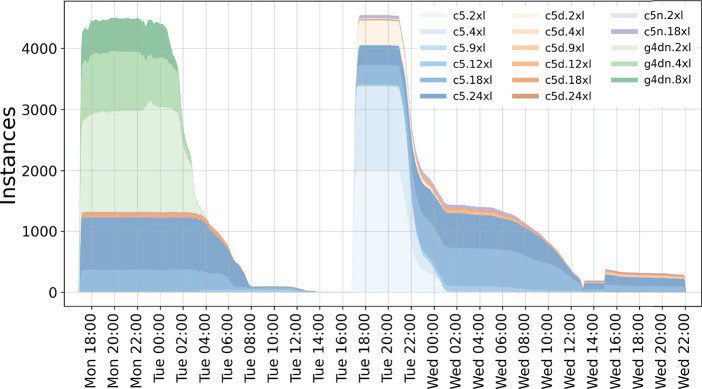
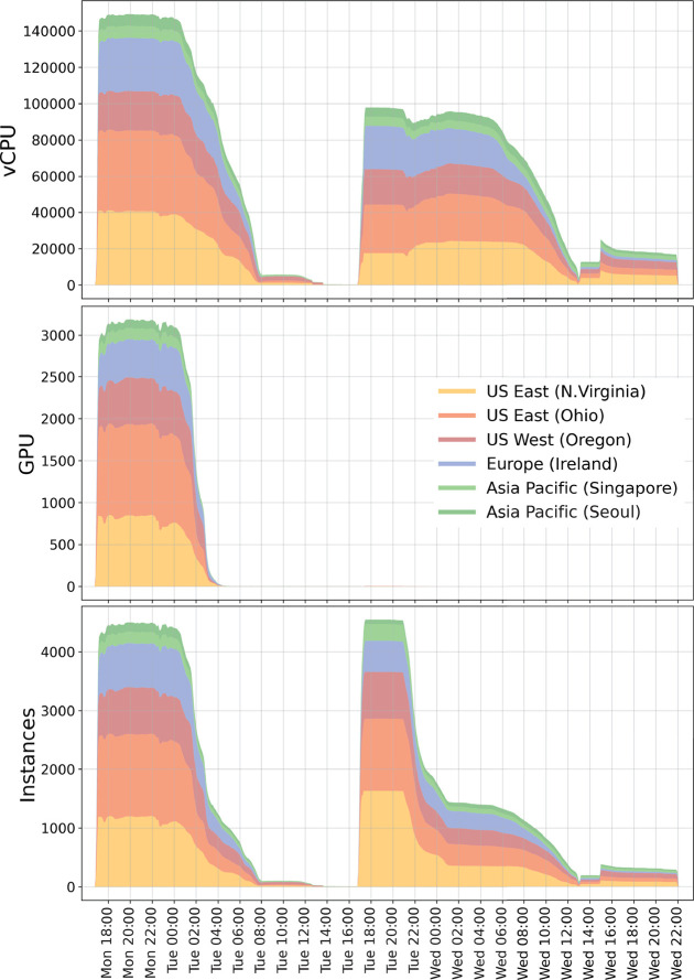
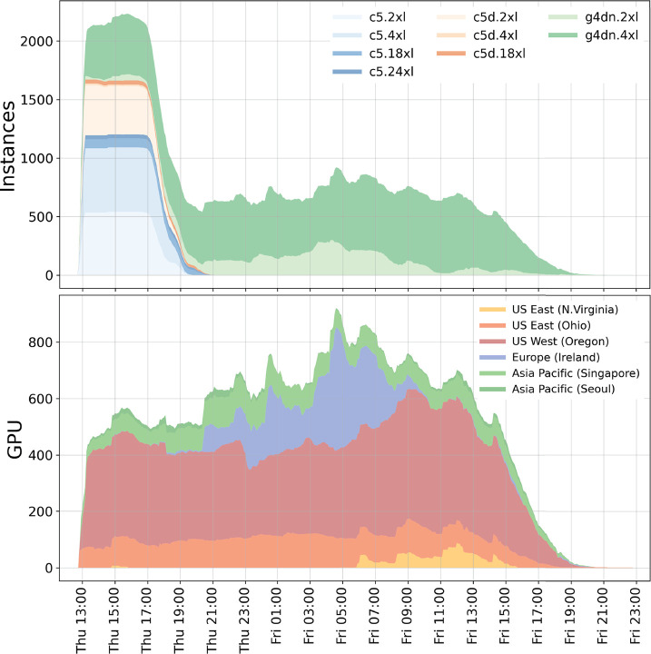
We assess costs and efficiency of state-of-the-art high-performance cloud computing and compare the results to traditional on-premises compute clusters. Our use case is atomistic simulations carried out with the GROMACS molecular dynamics (MD) toolkit with a particular focus on alchemical protein-ligand binding free energy calculations. We set up a compute cluster in the Amazon Web Services (AWS) cloud that incorporates various different instances with Intel, AMD, and ARM CPUs, some with GPU acceleration. Using representative biomolecular simulation systems, we benchmark how GROMACS performs on individual instances and across multiple instances. Thereby we assess which instances deliver the highest performance and which are the most cost-efficient ones for our use case. We find that, in terms of total costs, including hardware, personnel, room, energy, and cooling, producing MD trajectories in the cloud can be about as cost-efficient as an on-premises cluster given that optimal cloud instances are chosen. Further, we find that high-throughput ligand-screening can be accelerated dramatically by using global cloud resources. For a ligand screening study consisting of 19 872 independent simulations or ∼200 μs of combined simulation trajectory, we made use of diverse hardware available in the cloud at the time of the study. The computations scaled-up to reach peak performance using more than 4 000 instances, 140 000 cores, and 3 000 GPUs simultaneously. Our simulation ensemble finished in about 2 days in the cloud, while weeks would be required to complete the task on a typical on-premises cluster consisting of several hundred nodes.


Conflict of interest statement

The authors declare the following competing financial interest(s): Christian Kniep, Austin Cherian, and Ludvig Nordstrom are employees of Amazon.com, Inc.

Figures

Figure 1
Figure 1
HyperBatch-based setup distributes all 19 872 GROMACS jobs globally. An illustrative lifetime of a job follows the steps ①···⑧ and is described in section 3.4 of the text.
Figure 2
Figure 2
Example of a Docker file for a GPU image. From the Docker files multiple Docker container images are compiled (one for each architecture) that are loaded from the Amazon ECR by the instances.
Figure 3
Figure 3
Perl script used to launch each of the 19 872 jobs (first part).
Figure 4
Figure 4
Perl script used to launch each of the 19 872 jobs (cont’d).
Figure 5
Figure 5
Performance, costs, and cost-efficiency for GROMACS simulations on various AWS instance types. GROMACS 2020 performance as a function of the on-demand instance costs ($/h) for the MEM (circles), RIB (stars), and PEP (triangles) benchmark on CPU (open symbols) and GPU instances (filled symbols). Separate symbols indicate single-instances; connected symbols show the parallel scaling across multiple instances.
Figure 6
Figure 6
Costs and cost-efficiency of a compute node in an owned cluster compared to a cloud instance with similar GROMACS performance over 3 years. Top panel: Violet bars show costs of AWS g5.2xl instances (producing 7.55 ns/d of RIB trajectory), which offer one of the highest performance-to-price ratios for GROMACS (compare Figure 5), in individual blocks of one year. Bar A shows the fixed costs for buying a consumer GPU node tailored to GROMACS within the thick black line (broken down into individual hardware components) plus the yearly recurring costs (mainly energy) for three years. This node (E5-2630v4 CPU plus RTX 2080 GPU) produces 5.9 ns/d of RIB trajectory. Bar B shows the average costs using an AWS Spot instance. Bar C shows the costs when reserving the AWS instance and paying up front. Bar D is the same as bar A, but using a 4 U node with a professional GPU (e.g., Quadro P6000). Bars A–D in the lower panel show the resulting RIB trajectory costs for the nodes shown in the top panel, for a service life of three years.
Figure 7
Figure 7
Performance improvements of GROMACS 2021 for free energy calculations on GPUs. For three different MD systems (colors) with free energy perturbation turned on, the bars compare GROMACS 2021 and 2020 performances on a p3.2xl instance.
Figure 8
Figure 8
Costs and time needed to compute one FE difference. Diamonds show the costs to compute one FE difference (using Spot pricing) versus the time-to-solution for various instance types (colors) for the c-Met system. In addition to c-Met, HIF-2α is shown at the lower left end of each colored line, and SHP-2 at the upper right end. The gray square shows costs and timings for a consumer GPU node specifically tuned for GROMACS simulations, as discussed in section 4.2 and shown in Figure 6A.
Figure 9
Figure 9
Usage of global compute resources for the first ligand screening study aimed to optimize time-to-solution. Colors show the various instances that were in use globally during the 3 days of the ensemble run.
Figure 10
Figure 10
Usage of global compute resources for the first ligand screening study aimed to optimize time-to-solution. Compute resources (split into regions) allocated for the ensemble run over time. Top, vCPUs; middle, GPU instances; bottom, number of instances.
Figure 11
Figure 11
Usage of global compute resources for the second ligand screening study aimed at optimizing cost-efficiency. Top, allocated instance types over time; bottom, GPU instances allocated in the different regions.

References

    1. Baumann H. M.; Gapsys V.; de Groot B. L.; Mobley D. L. J. Phys. Chem. B 2021, 125, 4241–4261. 10.1021/acs.jpcb.0c10263. - DOI - PMC - PubMed
    1. Khalak Y.; Tresadern G.; Aldeghi M.; Baumann H. M.; Mobley D. L.; de Groot B. L.; Gapsys V. Chem. Sci. 2021, 12, 13958–13971. 10.1039/D1SC03472C. - DOI - PMC - PubMed
    1. Wang L.; Wu Y.; Deng Y.; Kim B.; Pierce L.; Krilov G.; Lupyan D.; Robinson S.; Dahlgren M. K.; Greenwood J.; Romero D. L.; Masse C.; Knight J. L.; Steinbrecher T.; Beuming T.; Damm W.; Harder E.; Sherman W.; Brewer M.; Wester R.; Murcko M.; Frye L.; Farid R.; Lin T.; Mobley D. L.; Jorgensen W. L.; Berne B. J.; Friesner R. A.; Abel R. J. Am. Chem. Soc. 2015, 137, 2695–2703. 10.1021/ja512751q. - DOI - PubMed
    1. Schindler C. E. M.; Baumann H.; Blum A.; Böse D.; Buchstaller H.-P.; Burgdorf L.; Cappel D.; Chekler E.; Czodrowski P.; Dorsch D.; Eguida M. K. I.; Follows B.; Fuchß T.; Grädler U.; Gunera J.; Johnson T.; Jorand Lebrun C.; Karra S.; Klein M.; Knehans T.; Koetzner L.; Krier M.; Leiendecker M.; Leuthner B.; Li L.; Mochalkin I.; Musil D.; Neagu C.; Rippmann F.; Schiemann K.; Schulz R.; Steinbrecher T.; Tanzer E.-M.; Unzue Lopez A.; Viacava Follis A.; Wegener A.; Kuhn D. J. Chem. Inf. Model. 2020, 60, 5457–5474. 10.1021/acs.jcim.0c00900. - DOI - PubMed
    1. Gapsys V.; Pérez-Benito L.; Aldeghi M.; Seeliger D.; Van Vlijmen H.; Tresadern G.; de Groot B. L. Chem. Sci. 2020, 11, 1140–1152. 10.1039/C9SC03754C. - DOI - PMC - PubMed

Publication types