Catastrophic hydraulic failure and tipping points in plants

Abstract

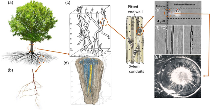
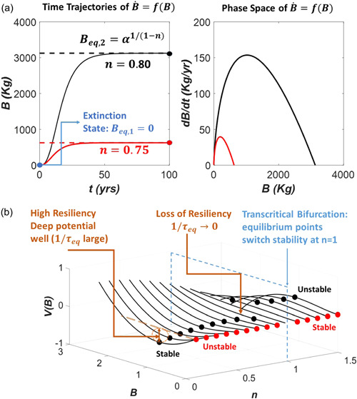
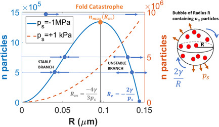
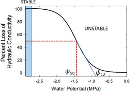
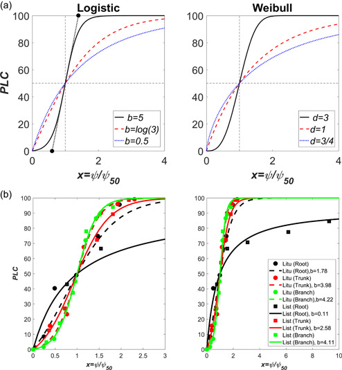
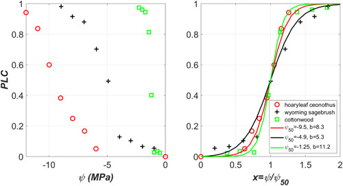
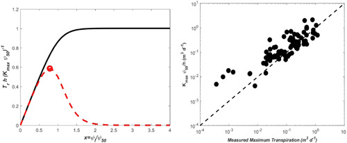
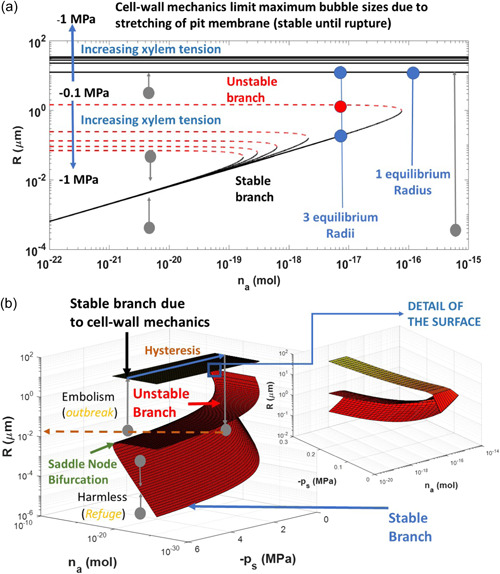
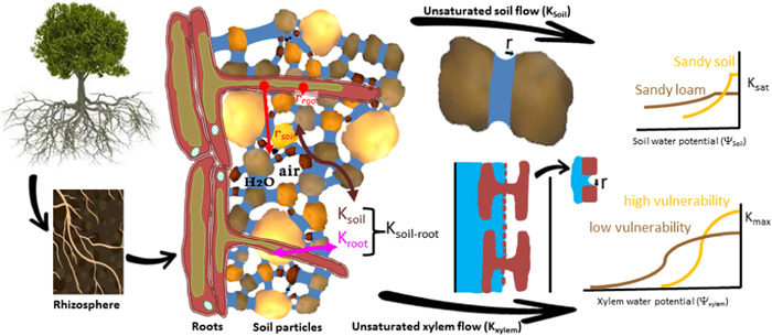
Water inside plants forms a continuous chain from water in soils to the water evaporating from leaf surfaces. Failures in this chain result in reduced transpiration and photosynthesis and are caused by soil drying and/or cavitation-induced xylem embolism. Xylem embolism and plant hydraulic failure share several analogies to 'catastrophe theory' in dynamical systems. These catastrophes are often represented in the physiological and ecological literature as tipping points when control variables exogenous (e.g., soil water potential) or endogenous (e.g., leaf water potential) to the plant are allowed to vary on time scales much longer than time scales associated with cavitation events. Here, plant hydraulics viewed from the perspective of catastrophes at multiple spatial scales is considered with attention to bubble expansion within a xylem conduit, organ-scale vulnerability to embolism, and whole-plant biomass as a proxy for transpiration and hydraulic function. The hydraulic safety-efficiency tradeoff, hydraulic segmentation and maximum plant transpiration are examined using this framework. Underlying mechanisms for hydraulic failure at fine scales such as pit membranes and cell-wall mechanics, intermediate scales such as xylem network properties and at larger scales such as soil-tree hydraulic pathways are discussed. Understudied areas in plant hydraulics are also flagged where progress is urgently needed.

Keywords: bifurcation; cavitation; cusp; embolism; fold; r-shaped curves; s-shaped curves; soil; transpiration; water potential; xylem.

Figure 1

Scales of hydraulic phenomena in woody plants addressed in this review and sections in which each scale is discussed; (a) whole tree scale (1–10 m; Sections 2, 6, and 7); (b) belowground properties of soil–root systems (µm–m; Sections 6 and 7); (c) early work on vessel networks from Zimmerman & Brown (1971) (xylem network scale; µm–m; Sections 4 and 7); (d) more recent work showing vessel network properties, yellow vessels are connected, blue vessels are unconnected, from Johnson et al. (2014); (e) visual observation of air‐seeding in a synthetic nanofluidic channel, from Duan et al. (2012); (f) refilling of an embolized vessel in grapevine, from Brodersen et al. (2018); (g) torus margo pit from Pseudotsuga menziesii, JC Domec, unpublished (panels e, f and g represent bubble and conduit scales; nm–µm; Sections 3, 5 and 7). Although panels (a)–(d) are representative of angiosperms, panel (g) represents the torus margo pits found in some angiosperms (mainly within the Oleaceae, Thymelaeaceae, Cannabaceae and Ulmaceae families; Dute, 2015) and in most conifer xylem which is discussed in Sections 5 and 7 and Box 4. All images are reproduced with permission. [Color figure can be viewed at wileyonlinelibrary.com]

Figure B1

(a) Illustration of the trajectories (left) and the phase‐space (right) for the VBE dynamical system for two control parameters: n = 0.75 and n = 0.80. The remaining parameters ($k_m$ = 0.6 per year, $\alpha$ = 5, and $B\left(0\right)$ = 0.1 kg) are the same for both cases. The two equilibrium points are also shown corresponding to $\mathit{dB}/\mathit{dt}=0$. The bifurcation analysis is conducted on the equilibrium biomass with the allometric scaling exponent n being the control parameter shown later in panel b. (b) The variations of the potential surface $V(B)$with B and n for $\alpha =0.95$. The two equilibrium points $B_{\mathrm{eq},2}={\alpha }^{1/(1-n)}$ and $B_{\mathrm{eq},1}=0$ are shown as black and red circles, respectively. Based on the convexity of V(B), the equilibrium state for $B_{\mathrm{eq},1}$ and $B_{\mathrm{eq},2}$ can be determined. For $n<1,B_{\mathrm{eq},2}$ is stable whereas $B_{\mathrm{eq},1}=0$ is unstable. For $n>1$, the stability of these equilibrium points reverses. Thus, a ‘catastrophe’ occurs when $n$ transitions from subunity to super‐unity (i.e., transcending or crossing a critical state). This bifurcation on the control parameter $n$ is known as ‘trans‐critical’ because no new equilibrium points are produced (or lost)—only their stability is exchanged with $n$ crossing a critical value of unity. This catastrophe is termed as ‘fold’ (Zeeman, 1976). The resiliency of this system is high because there is only one stable equilibrium point (instead of multiple stable equilibria). However, starting from $0<n<1$ and as the critical n = 1 is approached, the potential surface at $B_{\mathrm{eq},2}$ becomes shallower and shallower. At n = 1, the potential surface becomes entirely flat resulting in a collision between the two equilibrium points followed by a shift in their stability. That the potential is becoming shallower as the critical exponent n is approached is a signature of loss of resiliency—and can be used as an early warning signal of an impending catastrophe (in this case, a zero above ground biomass, i.e., plant death). [Color figure can be viewed at wileyonlinelibrary.com]

Figure 2

Analysis of bubble stability represented by the number of initial molecules (n_i ) as a function of bubble radius ( R ) that can be accommodated under two xylem pressures (p_s ) using the formulation in Konrad and Roth–Nebelsick (2003). When ${n_i<n}_{\max }$ and ${R<R}_{\mathrm{e}}$, the bubble remains stable and harmless to the xylem (i.e., the initial bubble will grow or shrink to the stable branch). When ${n_i<n}_{\max }$ and ${R>R}_{\mathrm{e}}$, the bubble will grow and may burst. When ${n_i>n}_{\max }$, the bubble will rapidly grow and may burst. When p_s  > 0, there is no catastrophe and a single stable equilibrium exist (dashed line). When p_s  < 0, the catastrophe is of a ‘fold’ type with one stable (or attractive) branch and one repelling (or unstable) branch. The saddle point defining the fold catastrophe is the point (R _m , n _max). [Color figure can be viewed at wileyonlinelibrary.com]

Figure 3

A typical xylem vulnerability curve (VC) as a function of xylem tension (water potential). When xylem tension is increasing with increasing time, the percent loss of conductivity (PLC) = 0% is an ‘unstable equilibrium’ whereas infinite xylem tension leads to a stable equilibrium at PLC = 100%. The ψ ₅₀ and ψ ₁₂ are the xylem tensions at 50% and 12% loss of conductivity, respectively. Derivation of ψ ₁₂ follows Domec and Gartner (2001). At least one vessel member must be embolized to initiate small deviations from the zero‐water potential state. [Color figure can be viewed at wileyonlinelibrary.com]

Figure B2

(a) Illustration of how r‐shaped and s‐shaped PLC curves emerge from the simplified logistic (left) and Weibull (right) models for embolism spread with constant b (left) and constant $d$ (right). For $b\le \log \mathrm{}\left(3\right)$, the logistic PLC resembles an r‐shaped function whereas for $b>\log \mathrm{}\left(3\right)$, the PLC is s‐shaped. Likewise, for $d\le 1$, the PLC resembles an r‐shaped function whereas for $d>1$, the PLC is s‐shaped. The two closed circles (left panel) is the extrapolation of the line ${\mathit{PLC}}_{\mathit{lin}}(x)$ to PLC= 0 (air entry) and PLC = 1 (runaway cavitation) and the determination of their associated normalized tension $x$ from b only. (b) The organ‐specific vulnerability curves for two species—Liriodendron tulipifera (Litu) and Liquidambar styraciflua (List) for normalized tension. The branch and trunk vulnerability curves are s‐shaped and similar (left) whereas the root vulnerability curve for List is r‐shaped (right). The left plot is shown over a restricted range of x to illustrate the collapse of branch and trunk level vulnerability curves for the logistic curve whereas the right plot is intended to illustrate the r‐shaped root vulnerability curve for List. [Color figure can be viewed at wileyonlinelibrary.com]

Figure 4

Left: Variations of measured xylem vulnerability curves (VC) across three species ranging from desert shrubs to riparian trees (data digitized by us from Sperry, 2000). Right: The percent loss of conductivity (PLC) variations for normalized xylem pressure ($x=\psi /{\psi }_{50}$) along with the logistic fit to them yielding the ease of cavitation spread parameter $b$. Note the approximate collapse of the measured VCs with $x$ on a single curve where the remaining shape differences can be explained by b. [Color figure can be viewed at wileyonlinelibrary.com]

Figure B3

Left panel: Comparison between normalized transpiration $T_{r}h{\left(K_{\max }{\psi }_{50}\right)}^{-1}$ against normalized leaf tension $x={\psi }_l/{\psi }_{50}$ for the continuous tension distribution across the entire root‐xylem system (black solid) and the hydraulic segmentation limit where leaf tension dominates the entire hydraulic conductivity (red dashed). The same vulnerability curve is used in both calculations ($b=5$). In the latter case, a clear maximum transpiration emerges (open circle) at $x_m$ whereas in the continuous xylem tension case, it does not. Right panel: comparison between measured and modelled maximum transpiration (=$K_{\max }{\psi }_{50}{h}^{-1}$) multiplied by sapwood area over three orders of magnitude. The one‐to‐one line is also shown (dashed). The analysis is suggestive that a safety‐efficiency tradeoff can emerge between $K_{\max }$ and ${\psi }_{50}{h}^{-1}$ (i.e., a hydraulic gradient) when conditioned on maximum transpiration (coefficient of determination = 0.74). When the analysis is repeated per unit sapwood area, the conclusions are unaltered though the scatter is somewhat larger. The data set includes the following species: Acer saccharum, Betula papyrifera, Carapa procera, Cecropia longipes, Eucalyptus grandis, Eucalyptus regnans, Eucalyptus saligna, Fagus sylvatica, Larix cajanderi, Larix gmelinii, Liquidambar styraciflua, Liriodendron tulipifera, Picea mariana, Pinus banksiana, Pinus pinaster, Pinus radiata, Populus tremuloides Populus Sp., Pseudotsuga menziesii, Salix matsudana, Quercus alba, Quercus rubra, and Quercus petraea. [Color figure can be viewed at wileyonlinelibrary.com]

Figure B4

(A) Bifurcation diagram shown in two‐dimensions (equilibrium bubble radius R vs. $n_a$) with variations in $p_s$ featured as multiple curves instead of a separate dimension illustrating the genesis of a cusp catastrophe. The equilibrium points are derived from the simplified sextic equation in the limit of large and small radii. The large radii equilibria corresponding to embolism are shown as horizontal lines. Note that this large R equilibria are independent of $n_a.$ The remaining two equilibria only exist for $n_a<n_{\max }$, where $n_{\max }$ decreases with increasing $p_s$. (b) Bifurcation diagram obtained by numerically solving the sextic equation at equilibrium when net forces acting on the bubble are in balance. This diagram reveals the cusp catastrophe surface along the two control parameters: initial (or background) xylem pressure and number of air molecules introduced into the bubble. The diagram resembles the cusp catastrophe studied for the spruce budworm dynamical system. The lower equilibrium radii forming the stable branch delineates harmless bubbles (resembling the refuge zone in the spruce budworm system) and the large radii stable equilibrium branch delineates embolism (associated with outbreak for the spruce budworm system). The saddle node bifurcation that forms in the absence of cell‐wall mechanics constraints (see Section 3) and the hysteresis loop along the cusp surface are also shown. Note that the radii associated with the upper stable branch are not sensitive to the number of air molecules except at very low xylem pressure (see detail). [Color figure can be viewed at wileyonlinelibrary.com]

Figure 5

A conceptual representation of the contributions and the changes in soil (K _soil) and root hairs (K _root) hydraulic conductivity to rhizosphere conductance (K _soil‐root). Water (blue) in soil is held by capillary forces in pore space (radius r) under negative pressure due to surface tension. As soil dries, the soil water potential ($\mathrm{\psi }$ _soil ) becomes more negative and air replaces the water‐filled pore space (i.e., degree of saturation becomes smaller). Consequently, soil conductivity at saturation (K _sat) declines rapidly with $\mathrm{\psi }$ _soil dependently of soil texture, with sandy (porous soils) having higher K _sat, and being more sensitive to $\mathrm{\psi }$ _soil than for example sandy loam. Similarly, water in root xylem is also held at the interface of inter‐conduit pits by capillary forces and as xylem water potential ($\mathrm{\psi }$ _xylem) decreases air‐seeding occurs (Figure 1e), leading to an embolized conduit whose hydraulic conductivity declines from its maximum or fully hydrated values (K _max). Roots with high vulnerability to embolism have generally higher K _max, but analogous to porous soils, are also more sensitive to negative $\mathrm{\psi }$ _xylem than roots with low vulnerability because of larger pit membrane pores. r _root and r _soil are root radius and the radial distance from the centre of the roots to the mean distance between roots, respectively. [Color figure can be viewed at wileyonlinelibrary.com]

Figure B5

Simulated changes in the percent loss of root to leaf conductance (K _root–leaf that corresponds to whole plant xylem characterized here by a ${\psi }_{50\_\text{plant}}$, that is, a mean water potential of −3 MPa inducing 50% loss of plant conductivity) and in the percent loss of soil to leaf conductance (K _soil‐leaf, i.e., vulnerability curves of the whole soil–plant hydraulic pathway) as soil dries in different soils and with root to leaf area ratios (R/L) of 1 (a) and 7 (b). [Color figure can be viewed at wileyonlinelibrary.com]

Figure B6

Simulated changes in relative transpiration and in the proportion of the soil to leaf hydraulic resistance (1/K _soil–leaf) located in the rhizosphere (1/K _soil–root, Figure 5) in different soils and with root area to leaf area ratios (R/L) of 1 (light blue or light red) or 7 (dark blue or dark red). Highlighted blue or red areas on each curve represent the range in critical soil water potentials (critical ${\psi }_{\mathrm{soil}}$) at which plant system experiences a transition from plant‐controlled to soil‐controlled fluxes or in other words when rhizosphere rather than xylem becomes more limiting for plant transpiration. For example, on sandy soil, critical ${\psi }_{\mathrm{soil}}$ decreased from −0.1 to −0.7 MPa when R/L increased from 1 to 7. Note that for the loam site critical ${\psi }_{\mathrm{soil}}$ at a R/L = 7 was <−10 MPa and is not represented in the figure. [Color figure can be viewed at wileyonlinelibrary.com]

Figure 6

(a) Xylem model network on a 100 × 100 grid. Vertical (black) lines correspond to vessels made up of stacked vessel elements. In this case, the xylem segment is 200 mm long. Horizontal (red) lines correspond to pit membranes (simple pits in the case of angiosperms). For easier visualization of the pit membranes that have negligible thickness compared to vessel lengths, horizontal grid lines are not to scale. Some vessels conduct more xylem water than others do, and in this example, the ones located in the ‘dead end’ as represented above conduct a relatively negligible amount of water. Simulation of an air injection experiment with two initial random embolisms in each cluster (blue) leaving other vessels isolated (magenta) is represented in (b). As air pressure is increased incrementally, initial embolisms propagate and nine embolized vessels (as opposed to 4 in b) are visible in (c). Simulations continues until both clusters becomes completely disconnected and non‐conducting (d). Panel (e) shows a cross section of a Quercus root with yellow ovals indicating vessels that are connected (represented as red horizontal lines in panel (a); for more information, see Johnson et al., 2014). Scale bar represents 500 µm. [Color figure can be viewed at wileyonlinelibrary.com]

Figure 7

The percent loss of hydraulic conductivity (PLC) of the xylem network earlier shown (filled squares) against xylem tension. To eliminate the effect of random initial embolism locations, 40 air‐injection simulations were performed and averaged. Logistic and Weibull fits to VCs are shown for reference. Vertical bars represent variability corresponding to initial condition sensitivity. No statistically significant difference between logistic and Weibull were apparent in this case though the Weibull shape better captures the simulation outcome at low xylem pressures. The estimated xylem pressure at which ${\psi }_P$ _‐50 occurred are also compared well with measured ${\psi }_P$ _‐50 in a similar network (Wheeler et al., 2005). [Color figure can be viewed at wileyonlinelibrary.com]

References

1. Adams, H.D. , Zeppel, M.J. , Anderegg, W.R. , Hartmann, H. , Landhäusser, S.M. , Tissue, D.T. et al. (2017) A multi‐species synthesis of physiological mechanisms in drought‐induced tree mortality. Nature Ecology and Evolution, 1, 1285–1291. - PubMed
1. Albuquerque, C. , Scoffoni, C. , Brodersen, C.R. , Buckley, T.N. , Sack, L. & McElrone, A.J. (2020) Coordinated decline of leaf hydraulic and stomatal conductances under drought is not linked to leaf xylem embolism for different grapevine cultivars. Journal of Experimental Botany, 71, 7286–7300. - PubMed
1. Allen, C.D. , Breshears, D.D. & McDowell, N.G. (2015) On underestimation of global vulnerability to tree mortality and forest die‐off from hotter drought in the Anthropocene. Ecosphere, 6, 1–55.
1. Allen, C.D. , Macalady, A.K. , Chenchouni, H. , Bachelet, D. , McDowell, N. , Vennetier, M. et al. (2010) A global overview of drought and heat‐induced tree mortality reveals emerging climate change risks for forests. Forest Ecology and Management, 259, 660–684.
1. Anfodillo, T. , Carraro, V. , Carrer, M. , Fior, C. & Rossi, S. (2006) Convergent tapering of xylem conduits in different woody species. New Phytologist, 169, 279–290. - PubMed
Publication types
LinkOut - more resources