A spatially aware likelihood test to detect sweeps from haplotype distributions

Abstract

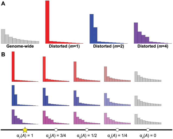
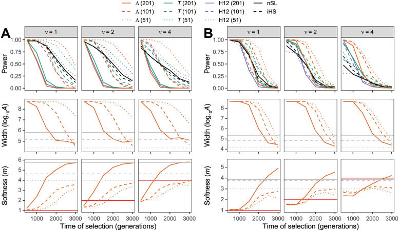
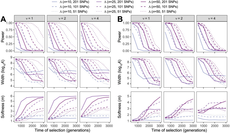
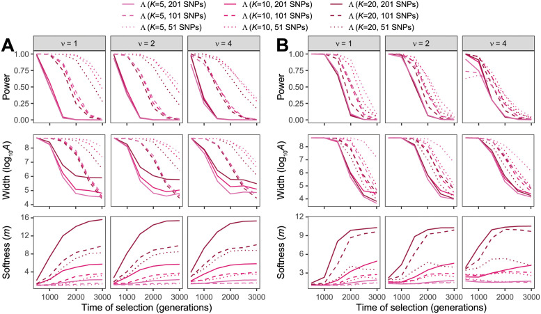
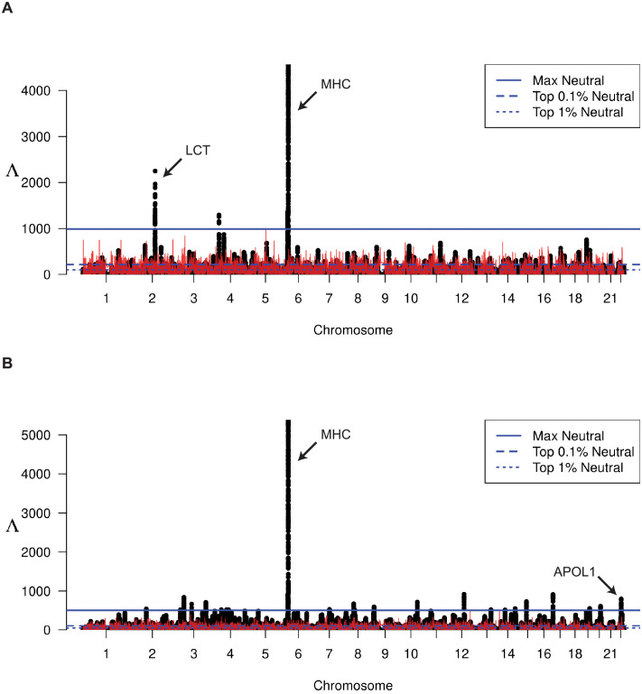
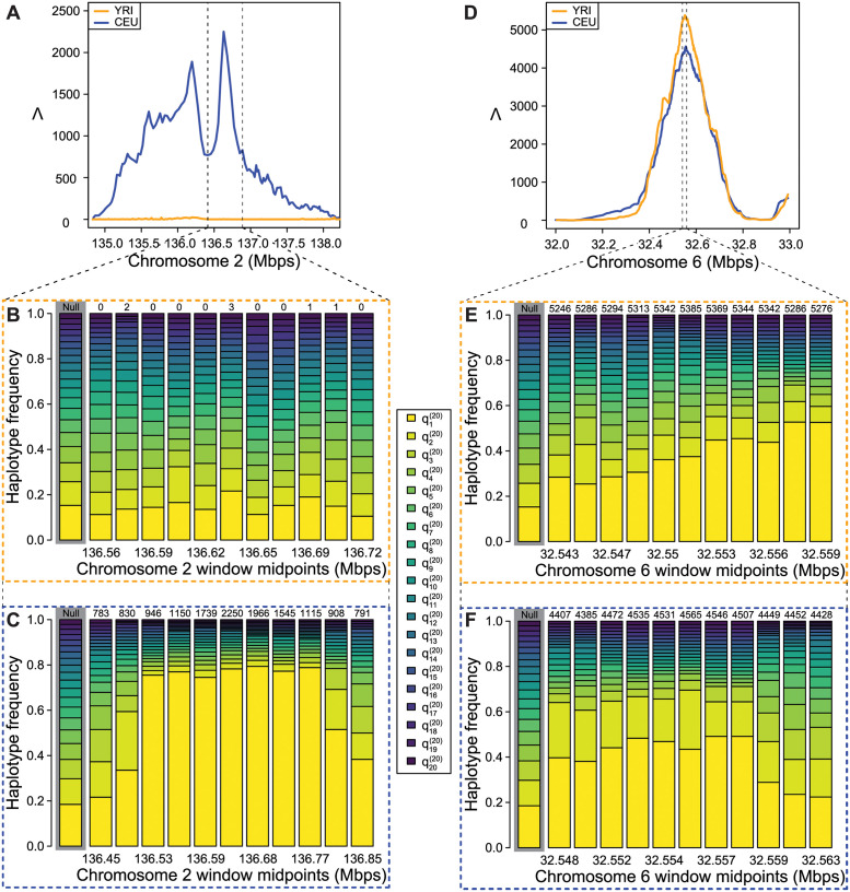
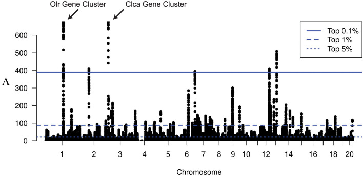
The inference of positive selection in genomes is a problem of great interest in evolutionary genomics. By identifying putative regions of the genome that contain adaptive mutations, we are able to learn about the biology of organisms and their evolutionary history. Here we introduce a composite likelihood method that identifies recently completed or ongoing positive selection by searching for extreme distortions in the spatial distribution of the haplotype frequency spectrum along the genome relative to the genome-wide expectation taken as neutrality. Furthermore, the method simultaneously infers two parameters of the sweep: the number of sweeping haplotypes and the "width" of the sweep, which is related to the strength and timing of selection. We demonstrate that this method outperforms the leading haplotype-based selection statistics, though strong signals in low-recombination regions merit extra scrutiny. As a positive control, we apply it to two well-studied human populations from the 1000 Genomes Project and examine haplotype frequency spectrum patterns at the LCT and MHC loci. We also apply it to a data set of brown rats sampled in NYC and identify genes related to olfactory perception. To facilitate use of this method, we have implemented it in user-friendly open source software.

Fig 1. Schematic of the saltiLASSI mixture model framework.

(A) Generation of distorted haplotype frequency spectra (HFS) for m = 1 (red), 2 (blue), and 4 (purple) sweeping haplotypes from a genome-wide (gray) neutral HFS under the LASSI framework of [13]. (B) Generation of spatially-distorted HFS under the saltiLASSI framework for a window i (white circles) with increasing distance from the sweep location (yellow star). When the window is on top of the sweep location, the HFS is identical to the distorted LASSI HFS, and α_i(A) = 1. When a window is far from the sweep location, the HFS is identical to the genome-wide (neutral) HFS, and α_i^⋆ (A) = 0. For windows at intermediate distances from the sweep location, the HFS is a mixture of the distorted and genome-wide HFS, with the distorted HFS contributing α_i(A) and the genome-wide HFS contributing 1 − α_i(A). We show example spectra at windows a, b, c, and d that are of increasing distances from the sweep location i^⋆, with i^⋆ < a < b < c < d.

Fig 2. Performance of detecting and characterizing sweeps.

Performance for applications of Λ, T, and H12 with windows of size 51, 101, and 201 SNPs, as well nS_L and iHS under simulations of (A) a constant-size demographic history or (B) the human central European (CEU) demographic history of [34]. Results are based on a sample of n = 50 diploid individuals and the haplotype frequency spectra for the Λ and T statistics truncated at K = 10 haplotypes. (Top row) Power at a 1% false positive rate as a function of selection start time. (Middle row) Estimated sweep width illustrated by mean estimated genomic size influenced by the sweep (${\text{log}}_{10}\widehat{A}$) as a function of selection start time. Gray solid, dashed, and dotted horizontal lines are the corresponding mean ${\text{log}}_{10}\widehat{A}$ values for Λ applied to neutral simulations. (Bottom row) Estimated sweep softness illustrated by mean estimated number of sweeping haplotypes ($\widehat{m}$) as a function of selection start time. Gray solid, dashed, and dotted horizontal lines are the corresponding mean $\widehat{m}$ values for Λ applied to neutral simulations, and the red solid horizontal lines correspond to the number of sweeping haplotypes ν ∈ {1, 2, 4} assumed in sweep simulations. Sweep scenarios consist of hard (ν = 1) and soft (ν ∈ {2, 4}) sweeps with per-generation selection coefficient of s = 0.1 that started at t ∈ {500, 1000, 1500, 2000, 2500, 3000} generations prior to sampling. Results expanded across wider range of simulation settings can be found in S1–S3 and S7–S9 Figs as well as results for application to unphased multilocus genotype data in S4–S6 and S10–S12 Figs.

Fig 3. Performance of detecting and characterizing sweeps.

Performance for applications of Λ with windows of size 51, 101, and 201 SNPs under simulations of (A) a constant-size demographic history or (B) the human central European (CEU) demographic history of [34] and sample size of n ∈ {10, 25, 50} diploid individuals. Results are based on the haplotype frequency spectra for the Λ statistic truncated at K = 10 haplotypes. (Top row) Power at a 1% false positive rate as a function of selection start time. (Middle row) Estimated sweep width illustrated by mean estimated genomic size influenced by the sweep (${\text{log}}_{10}\widehat{A}$) as a function of selection start time. (Bottom row) Estimated sweep softness illustrated by mean estimated number of sweeping haplotypes ($\widehat{m}$) as a function of selection start time. Sweep scenarios consist of hard (ν = 1) and soft (ν ∈ {2, 4}) sweeps with per-generation selection coefficient of s = 0.1 that started at t ∈ {500, 1000, 1500, 2000, 2500, 3000} generations prior to sampling. Results expanded across wider range of simulation settings can be found in S20–S22 and S26–S28 Figs as well as results for application to unphased multilocus genotype data in S23–S25 and S29–S31 Figs.

Fig 4. Performance of detecting and characterizing sweeps.

Performance for applications of Λ with windows of size 51, 101, and 201 SNPs under simulations of (A) a constant-size demographic history or (B) the human central European (CEU) demographic history of [34] and the haplotype frequency spectra for the Λ statistic truncated at K ∈ {5, 10, 20} haplotypes. Results are based on a sample of n = 50 diploid individuals. (Top row) Power at a 1% false positive rate as a function of selection start time. (Middle row) Estimated sweep width illustrated by mean estimated genomic size influenced by the sweep (${\text{log}}_{10}\widehat{A}$) as a function of selection start time. (Bottom row) Estimated sweep softness illustrated by mean estimated number of sweeping haplotypes ($\widehat{m}$) as a function of selection start time. Sweep scenarios consist of hard (ν = 1) and soft (ν ∈ {2, 4}) sweeps with per-generation selection coefficient of s = 0.1 that started at t ∈ {500, 1000, 1500, 2000, 2500, 3000} generations prior to sampling. Results expanded across wider range of simulation settings can be found in S32–S34 and S38–S40 Figs as well as results for application to unphased multilocus genotype data in S35–S37 and S41–S43 Figs.

Fig 5. Manhattan plot of Λ-statistics.

For the (A) CEU and (B) YRI populations from the 1000 Genomes Project. Each point represents a single 201-SNP window along the genome. Horizontal lines represent the top 1%, top 0.1%, and maximum observed Λ statistic across all windows in demography-matched neutral simulations. Red line indicates the maximum observed Λ among 100 replicate simulations at that location in the genome.

Fig 6. Detailed illustration of Λ statistics and haplotype frequency spectra in CEU and YRI.

(A) Λ plotted in the LCT region, vertical dotted lines indicate zoomed region shown in (B) and (C). (B) YRI empirical HFS for 11 windows in the LCT region. (C) CEU empirical HFS for 11 windows in the LCT region. (D) Λ plotted in the MHC region, vertical dotted lines indicate zoomed region shown in (E) and (F). (E) YRI empirical HFS for 11 windows in the MHC region. (F) CEU empirical HFS for 11 windows in the MHC region. In (B), (C), (E), and (F), numbers above HFS are Λ values for the window rounded to the nearest whole number, and the genome-wide average HFS is highlighted in grey. $q_i^{20}$ is the frequency of the ith most common haplotype truncated to K = 20.

Fig 7. Manhattan plot of Λ-statistics for the New York City rat population.

Each point represents a single 201-SNP window along the genome. Horizontal lines represent the top 5%, top 1%, and top 0.1% observed Λ statistic across all windows in the genome.

References

1. Przeworski M. The Signature of Positive Selection at Randomly Chosen Loci. Genetics. 2002;160:1179–1189. doi: 10.1093/genetics/160.3.1179 - DOI - PMC - PubMed
1. Hermisson J, Pennings P. Soft sweeps. Genetics. 2005;4:2335–2352. doi: 10.1534/genetics.104.036947 - DOI - PMC - PubMed
1. Pennings P, Hermisson J. Soft Sweeps II—Molecular Population Genetics of Adaptation from Recurrent Mutation or Migration. Mol Biol Evol. 2006;23:1076–1084. doi: 10.1093/molbev/msj117 - DOI - PubMed
1. Sabeti P, Reich D, Higgins J, Levine H, Richter D, Schaffner S, et al.. Detecting recent positive selection in the human genome from haplotype structure. Nature. 2002;419:832–837. doi: 10.1038/nature01140 - DOI - PubMed
1. Voight B, Kudaravalli S, Wen X, Pritchard J. A Map of Recent Positive Selection in the Human Genome. PLoS Biol. 2006;4:e72. doi: 10.1371/journal.pbio.0040072 - DOI - PMC - PubMed
Publication types