A real-time data assimilative forecasting system for animal tracking

Abstract

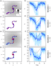
Monitoring technologies now provide real-time animal location information, which opens up the possibility of developing forecasting systems to fuse these data with movement models to predict future trajectories. State-space modeling approaches are well established for retrospective location estimation and behavioral inference through state and parameter estimation. Here we use a state-space model within a comprehensive data assimilative framework for probabilistic animal movement forecasting. Real-time location information is combined with stochastic movement model predictions to provide forecasts of future animal locations and trajectories, as well as estimates of key behavioral parameters. Implementation uses ensemble-based sequential Monte Carlo methods (a particle filter). We first apply the framework to an idealized case using a nondimensional animal movement model based on a continuous-time random walk process. A set of numerical forecasting experiments demonstrates the workflow and key features, such as the online estimation of behavioral parameters using state augmentation, the use of potential functions for habitat preference, and the role of observation error and sampling frequency on forecast skill. For a realistic demonstration, we adapt the framework to short-term forecasting of the endangered southern resident killer whale (SRKW) in the Salish Sea using visual sighting information wherein the potential function reflects historical habitat utilization of SRKW. We successfully estimate whale locations up to 2.5 h in advance with a moderate prediction error (<5 km), providing reasonable lead-in time to mitigate vessel-whale interactions. It is argued that this forecasting framework can be used to synthesize diverse data types and improve animal movement models and behavioral understanding and has the potential to lead to important advances in movement ecology.

Keywords: animal movement; continuous-time correlated random walk; data assimilation; ecological forecasting; particle filter; potential function; southern resident killer whale; state augmentation; state-space models; trajectory prediction; whale collision avoidance.

FIGURE 1

Schematic of DA cycle used for animal prediction system. It shows a single‐stage transition of this probabilistic system from time t − 1 to t and how it toggles between movement model forecasts and particle‐filter‐based assimilation of incoming observations (see Data assimilation for further details). Light and dark blue dots represent ensemble members (particles) at the nowcast and forecast steps, respectively. Red dots are the location observations, and red circles correspond to measurement errors. Assimilation and forward model prediction are symbolized by A and M, respectively.

FIGURE 2

Idealized example. (a, c, e, g) Observed (red dots) and predicted animal locations (blue dots are the ensemble median; light blue dots show full ensemble). The true animal track is shown (black line) along with initial position (black cross). In panels (a) and (e), the gray scale represents potential field reflecting animal's preferred habitat. Panels (a) and (c) present high‐quality location data (${\mathrm{\sigma }}_{\mathrm{\epsilon }}=0.1$, observations every time step), as opposed to panels (e) and (g), which present lower‐quality location data (${\mathrm{\sigma }}_{\mathrm{\epsilon }}=0.2$, observations every second time step). (b, d, f, h) Time‐varying estimates of velocity persistence parameter ϕ _t . The black lines show the true persistence velocity used for computing the true track (a sine wave) and estimation results (ensemble, light blue dots; ensemble median, blue dots; fitted smooth curve, blue lines). Note that spatial coordinates and time vectors are nondimensional.

FIGURE 3

(a) An n‐step ahead error forecast (root mean square error [RMSE]) of idealized example. (b) Heatmap representing relationship between behavioral parameter ϕ _t and n‐step ahead error forecast (RMSE) for Simulation 1 (low observation error ${\mathrm{\sigma }}_{\mathrm{\epsilon }}=0.1$, observations every time step, and drift term)

FIGURE 4

Assimilation experiment. (a) Visual observations of SRKW J pod on 18 August 2016 (white symbols with red outline) and predicted whale locations (blue dots, ensemble median). Solid red symbols represent starting (10:34 AM) and ending (4:00 PM) observations for day. Letters A to N designate the chronology of these observations, with A being the first observation. The gray scale represents the whale intensity field of J pod in August, expressed in log scale (from Watson et al. [2019]). (b, c) UTM easting and northing coordinates of whale locations, including ensembles (gray dots) and their median (blue dots). Symbols denote visual sighting location observations following panel (a).

FIGURE 5

Forecast experiment. (a) This follows Figure 4 except solid orange symbols represent first data point used for assimilation, and open symbols represent location observations used for n‐step ahead forecast validation (see Data assimilation for details). (b) Direct position error of forecast (km) against time. Symbols show discrepancy of ensemble median and observed location, with range being 5th and 95th percentiles of position error associated with full ensemble. (c–f) Kernel density estimates (KDE) of forecast probability density function (PDF) of whale locations up to 3.5 h ahead shown together with future observation

References

-
- Abrahms, B. , Welch H., Brodie S., Jacox M. G., Becker E. A., Bograd S. J., Irvine L. M., Palacios D. M., Mate B. R., and Hazen E. L.. 2019. “Dynamic Ensemble Models to Predict Distributions and Anthropogenic Risk Exposure for Highly Mobile Species.” Diversity and Distributions 25(8): 1182–93.
- Auger‐Méthé, M. , Newman K., Cole D., Empacher F., Gryba R., King A. A., Leos‐Barajas V., et al. 2020. “An Introduction to State‐Space Modeling of Ecological Time Series.” arXiv preprint arXiv:2002.02001.
- Barlow, D. R. , and Torres L. G.. 2021. “Planning Ahead: Dynamic Models Forecast Blue Whale Distribution with Applications for Spatial Management.” Journal of Applied Ecology 58(11): 2493–504.
- Brillinger, D. R. , Preisler H. K., Ager A. A., and Kie J.. 2012. “The Use of Potential Functions in Modelling Animal Movement.” In Selected Works of David Brillinger, edited by Guttorp P. and Brillinger D., 385–409. New York, NY: Springer.
Publication types
MeSH terms
Associated data
LinkOut - more resources
Full Text Sources