Multi-animal pose estimation, identification and tracking with DeepLabCut

Abstract

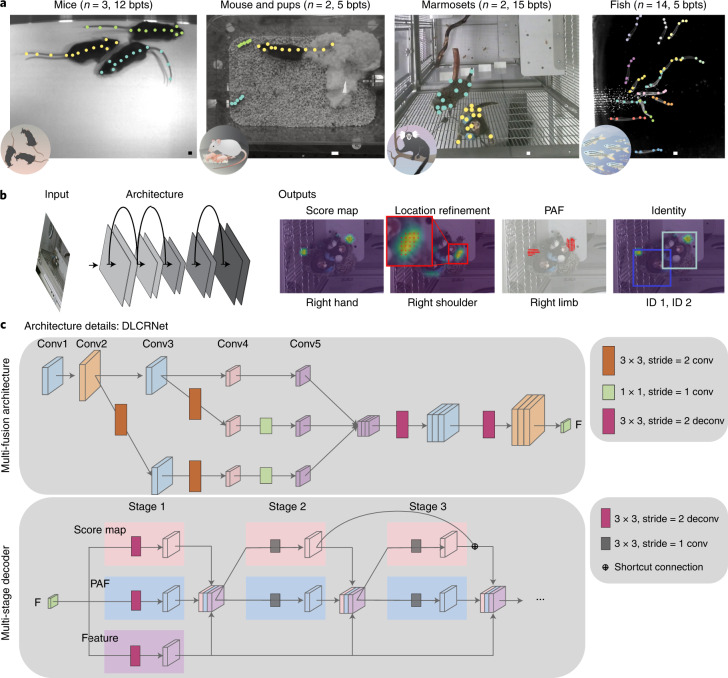
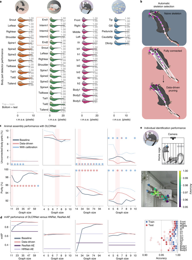
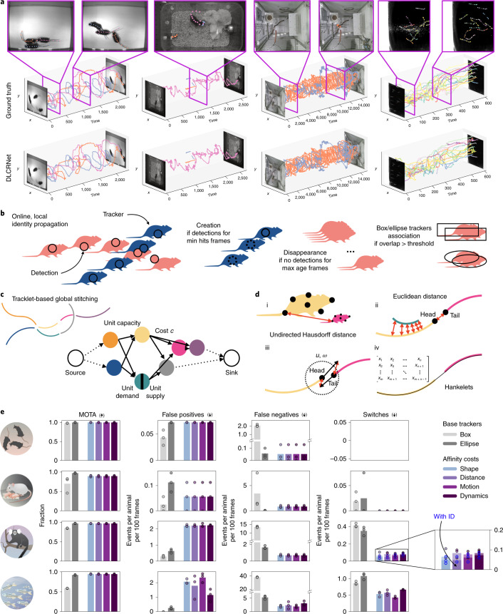
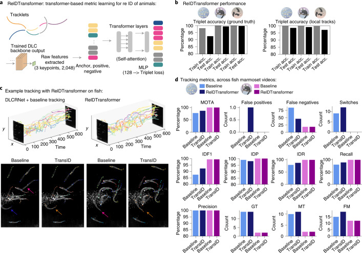
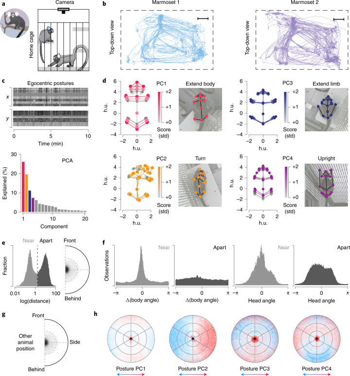
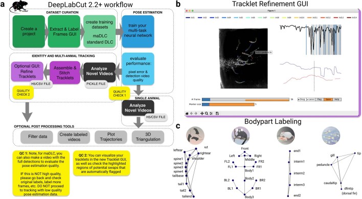
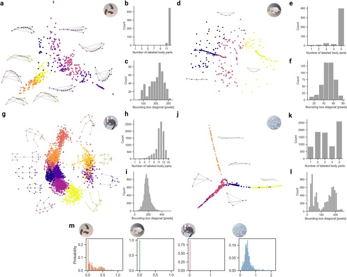
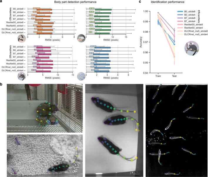
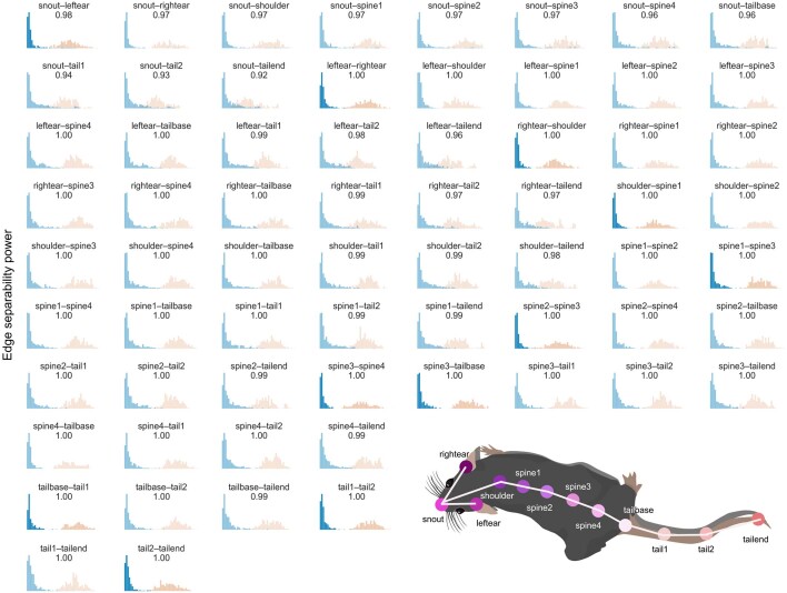
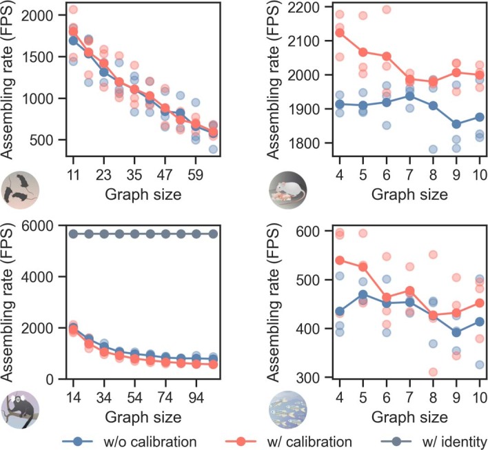
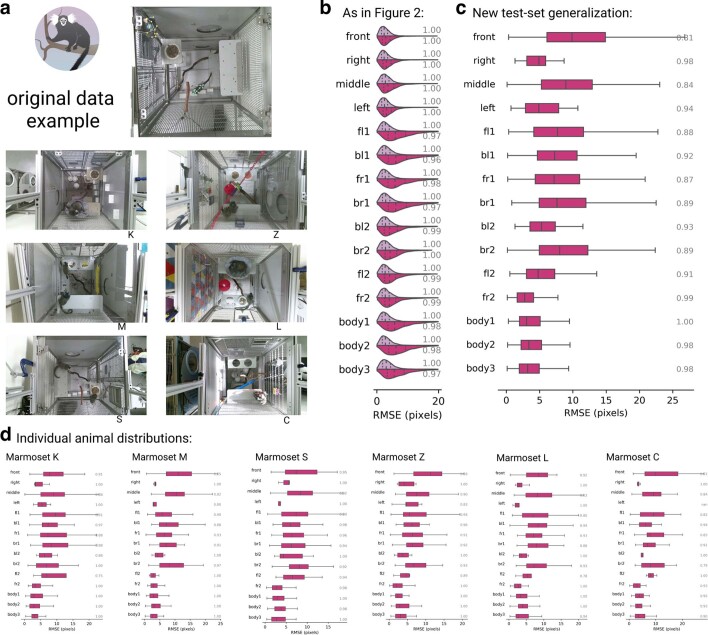
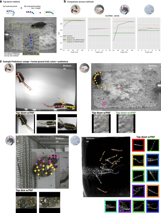
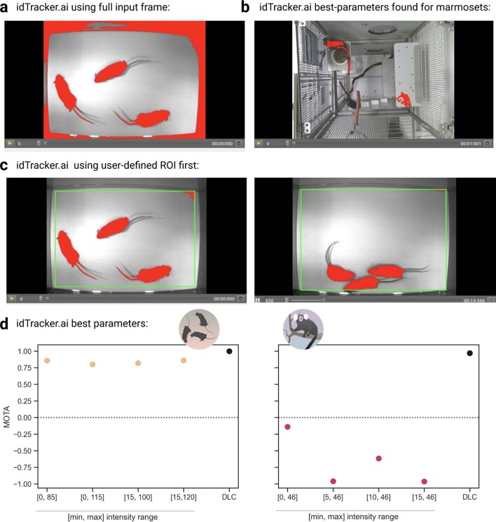
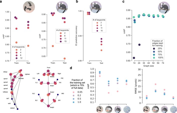
Estimating the pose of multiple animals is a challenging computer vision problem: frequent interactions cause occlusions and complicate the association of detected keypoints to the correct individuals, as well as having highly similar looking animals that interact more closely than in typical multi-human scenarios. To take up this challenge, we build on DeepLabCut, an open-source pose estimation toolbox, and provide high-performance animal assembly and tracking-features required for multi-animal scenarios. Furthermore, we integrate the ability to predict an animal's identity to assist tracking (in case of occlusions). We illustrate the power of this framework with four datasets varying in complexity, which we release to serve as a benchmark for future algorithm development.

Fig. 1. Multi-animal DeepLabCut architecture and benchmarking datasets.

a, Example (cropped) images with (manual) annotations for the four datasets: mice in an open field arena, parenting mice, pairs of marmosets and schooling fish. bpts, body parts. Scale bars, 20 pixels. b, A schematic of the general pose estimation module. The architecture is trained to predict the keypoint locations, PAFs and animal identity. Three output layers per keypoint predict the probability that a joint is in a particular pixel (score map) as well as shifts in relation to the discretized output map (location refinement field). Furthermore, PAFs predict vector fields encoding the orientation of a connection between two keypoints. Example predictions are overlaid on the corresponding (cropped) marmoset frame. The PAF for the right limb helps linking the right hand and shoulder keypoints to the correct individual. c, Our architecture contains a multi-fusion module and a multi-stage decoder. In the multi-fusion module, we add the high-resolution representation (conv2, conv3) to low-resolution representation (conv5). The features from conv2 and conv3 are downsampled by two and one 3 × 3 convolution layer, respectively to match the resolution of conv5. Before concatenation the features are downsampled by a 1 × 1 convolution layer to reduce computational costs and (spatially) upsampled by two stacked 3 × 3 deconvolution layers with stride 2. The multi-stage decoder predicts score maps and PAFs. At the first stage, the feature map from the multi-fusion module are upsampled by a 3 × 3 deconvolution layer with stride 2, to get the score map, PAF and the upsampled feature. In the latter stages, the predictions from the two branches (score maps and PAFs), along with the upsampled feature are concatenated for the next stage. We applied a shortcut connection between the consecutive stage of the score map. The shown variant of DLCRNet has overall stride 2 (in general, this can be modulated from 2 to 8).

Fig. 2. Multi-animal DeepLabCut keypoint detection and whole-body assembly performance.

a, Distribution of keypoint prediction error for DLCRNet_ms5 with stride 8 (70% train and 30% test split). Violin plots display train (top) and test (bottom) errors. Vertical dotted lines are the first, second and third quartiles. Median test errors were 2.69, 5.62, 4.65 and 2.80 pixels for the illustrated datasets, in order. Gray numbers indicate PCK. Only the first five keypoints of the parenting dataset belong to the pups; the 12 others are keypoints of the adult mouse. b, Illustration of our data-driven skeleton selection algorithm. Mouse cartoon adapted with permission from ref. under a Creative Commons licence (https://creativecommons.org/licenses/by/4.0/). c, Animal assembly quality as a function of part affinity graph (skeleton) size for baseline (user-defined) versus data-driven skeleton definitions. The top row displays the fraction of keypoints left unconnected after assembly, whereas the bottom row designates the accuracy of their grouping into distinct animals. The colored dots mark statistically significant interactions (two-way, repeated-measures ANOVA; see Supplementary Tables 1–4 for full statistics). Light red vertical bars highlight the graph automatically selected. d, mAP as a function of graph size. Shown on test data held out from 70% train and 30% test splits. The associative embedding method does not rely on a graph. The performance of MMPose’s implementation of ResNet-AE and HRNet-AE bottom-up variants is shown for comparison against our multi-stage architecture DLCRNet_ms5, here called Baseline. Data-driven is Baseline plus calibration method (one-way ANOVA show significant effects of the model: P values, tri-mouse 8.8 × 10⁻⁸, pups 6.5 × 10⁻¹³, marmosets 3.8 × 10⁻¹¹, fish 4.0 × 10⁻¹²). e, Marmoset ID–Example test image together with overlaid animal identity prediction accuracy per keypoint averaged over all test images and test splits. With ResNet50_stride8, accuracy peaks at 99.2% for keypoints near the head and drops to only 95.1% for more distal parts. In the lower panel, plus signs denote individual splits, circles show the averages.

Fig. 3. Linking whole-body assemblies across time.

a, Ground truth and reconstructed animal tracks (with DLCRNet and ellipse tracking), together with video frames illustrating representative scene challenges. b, The identities of animals detected in a frame are propagated across frames using local matching between detections and trackers (with costs, ‘motion’ for all datsets and ‘distance’ for fish). c, Tracklets are represented as nodes of a graph, whose edges encode the likelihood that the connected pair of tracklet belongs to the same track. d, Four cost functions modeling the affinity between tracklets are implemented: shape similarity using the undirected Hausdorff distance between finite sets of keypoints (i); spatial proximity in Euclidean space (ii); motion affinity using bidirectional prediction of a tracklet’s location (iii); and dynamic similarity via Hankelets and time-delay embedding of a tracklet’s centroid (iv). e, Tracklet stitching performance versus box and ellipse tracker baselines (arrows indicate if higher or lower number is better), using MOTA, as well as rates of false negative (FN), false positives (FP) and identity switch expressed in events per animal and per sequence of 100 frames. Inset shows that incorporating appearance/identity prediction in the stitching further reduces the number of switches and improves full track reconstruction. Total number of frames: tri-mouse, 2,330; parenting, 2,670; marmosets, 15,000 and fish, 601.

Fig. 4. Unsupervised reID of animals.

a, Schematic of the transformer architecture we adapted to take pose-tensor outputs of the DeepLabCut backbone. We trained it with triplets sampled from tracklets and tracks. b, Performance of the ReIDTransformer method on unmarked fish, mice and marked marmosets. Triplet accuracy (acc.) is reported for triplets sampled from ground truth (GT) tracks and local tracklets only. We used only the top 5% of the most crowded frames, as those are the most challenging. c, Example performance on the challenging fish data. Top: fish-identity-colored tracks. Time is given in frame number. Bottom: example frames (early versus later) from baseline or ReIDTransformer. Arrows highlight performance with ReIDTransformer: pink arrows show misses; orange shows correct ID across frames in ReIDTransformer versus blue to orange in baseline. d, Tracking metrics on the most crowded 5% of frames (30 frames for fish, 744 for marmosets, giving 420 fish targets and 1,488 marmoset targets); computed as described in Methods. IDF1, ID measure, global min-cost F1 score; IDP, ID measure, global min-cost precision; IDR, ID measures: global min-cost recall; Recall, number of detections over number of objects; Precision, number of detected objects over sum of detected and false positives; GT, number of unique objects; MT, mostly tracked and FM, number of fragmentations.

Fig. 5. Application to multi-marmoset social behaviors.

a, Schematic of the marmoset recording setup. b, Example tracks, 30 min plotted from each marmoset. Scale bars, 0.2 m. c, Example egocentric posture data, where the ‘Body2’ point is (0,0) and the angle formed by ‘Body1’ and ‘Body3’ is rotated to 0°. We performed principal component analysis on the pooled data of both marmosets for all data. d, Average postures along each principal component; note that only one side of the distribution is represented in the image (that is, 0 to 2 instead of −2 to 2). e, Histogram of log-distance between a pair of marmosets normalized to ear-center distance. f, Computed body angle versus observation count. g, Density plot of where another marmoset is located relative to marmoset 1. h, Postural principal components (from d) as a function of the relative location of the other marmoset. Thereby, each point represents the average postural component score for marmoset 1 when marmoset 2 is at that point. h.u., head units.

Extended Data Fig. 1. DeepLabCut 2.2 workflow.

(a) Multi-animal DeepLabCut2.2+ workflow. (b) An example screenshot of the Refine Tracklet GUI. We show the ellipse similarity score (black line), hand-noted GT switches in ID (blue), and additional frames in orange where the selected keypoint requires further examination. (c) Body part keypoint diagrams with names on the animal skeletons (see also Extended Data Figure 2).

Extended Data Fig. 2. Dataset characteristics and statistics.

For each datasets, normalized animal poses were clustered using K-means adapted for missing elements, and embedded non-linearly in 2D space via Isometric mapping (Tenenbaum et al. 2000). Embeedings as well as representative poses are shown for the tri-mouse dataset (a). Counts of labeled keypoints (b) and distribution of bounding box diagonal lengths (c). (d-l) show the same for the other three datsets. The Proximity Index (m) reflects the crowdedness of the various dataset scenes. Statistics were computed from the ground truth test video annotations. The mice and fish datasets are more cluttered on average than the pups and marmosets.

Extended Data Fig. 3. Performance of various DeepLabCut network architectures.

(a) Overall keypoint prediction errors of ResNets-50 and the EfficientNets backbones (B0/B7), DLCRNet at stride 4 and 8. Distribution of train and test errors are displayed as light and dark box plots, respectively. Box plots show median, first and third quartiles, with whiskers extending past the low and high quartiles to ± 1.5 times the interquartile range. All models were trained for 60k iterations. n=independent image samples as follows: for train∣test per dataset: 112∣49 (tri-mouse); 379∣163 (pups); 5316∣2278 (marmosets); 70∣30 (fish). (b): Images on held-out test data, where plus indicates human ground truth, and the circle indicates the model prediction (shown for ResNet50 with stride 8). (c): Marmoset identification train-test accuracy for various backbones.

Extended Data Fig. 4. Discriminability of part affinity fields.

Within- (pink) and between-animal (blue) affinity cost distributions for all edges of the mouse skeleton with DLCRNet_ms5. The saturated subplots highlight the 11 edges kept to form the smallest, optimal part affinity graph (see Fig. 2b). This is based on the separability power of an edge, that is, its ability to discriminate a connection between two keypoints effectively belonging to the same animal from the wrong ones, and reflected by the corresponding AUC scores (listed at the top of the subplots).

Extended Data Fig. 5. Average animal assembly speed in frames per second as a function of graph size.

Assembly rates vs. graphs size for the four datasets. Improving the assembly robustness via calibration with labeled data in large graphs incurs no extra computational cost at best, and a slowdown by 25% at worst; remarkably, it is found to accelerate assembly speed in small graphs. Relying exclusively on keypoint identity prediction results in average speeds of around 5600 frames per second, independent of graph size. Three timing experiments were run per graph size (lighter colored dots) and averages are shown. Note that assembling rates exclude CNN processing times. Speed benchmark was run on a workstation with an Intel(R) Core(TM) i9-10900X CPU 3.70GHz.

Extended Data Fig. 6. Performance on out of domain marmoset data.

(a) Example images from original dataset, and example generalization test images. (b) Median RMSE and PCK (gray numbers) for data and network (DLCRNet) as shown in Fig. 2a. (c) same, but on the generalization test images (n=300) (d) same but per cage as shown in a (n=30 test images per marmoset). Box plots show median, first and third quartiles, with whiskers extending past the low and high quartiles to ± 1.5 times the interquartile range.

Extended Data Fig. 7. Comparison of top-down methods with and without assembly.

(a) Schematics of top-down method with example images from the pup dataset, which consists of first detecting individuals and then performing pose prediction on each bounding box (plus is human ground truth, and the circle is bottom-up model (DLCRNet, stride 8, data-driven) predictions. (b) Performance mAP computed for top-down method with and without PAFs and bottom-up method (baseline, data-driven) as also shown in Fig. 2d. PAF vs. w/o PAF one-way ANOVA p-values, tri-mouse: 4.656e-11, pups: 3.62e-12, marmosets: 1.33e-28, fish: 1.645e-06). There were significant model effects across all datasets: one-way ANOVA p-values– tri-mouse: 4.13e-11, pups: 4.59e-25, marmosets: 3.04e-40, fish: 1.18e-14. (c) Example predictions within the smaller images (that is, bounded crops) from the top-down model (that is, w/PAF), and bottom-up predictions (full images, as noted).

Extended Data Fig. 8. Performance of idtracker.ai.

(a) Segmented regions (red) overlaid on example image in idtracker.ai GUI. Example how idtracker.ai fails to segment only the mice in the full data frame for tri-mouse and (b) in marmoset dataset. (c) Using the ROI selection feature, we could find mostly just mice. However, due to the inhomogeneous lighting, the segmentation is not error-free. (d) Result of a grid search to find optimal parameters for idtracker with MOTA scores on the same videos as shown in Fig. 3a,e; one-sided, one-sample T-tests indicated that idtracker.ai performed significantly worse than DeepLabCut in both datasets (tri-mouse: T=-11.03, p=0.0008, d=5.52; marmosets: T=-8.43, p=0.0018, d=4.22).

Extended Data Fig. 9. Parameter sensitivity: Evaluation of number of body parts, frames, and PAF sizes.

(a) The number of keypoints affects mAP; evaluated with ResNet50 stride8 on the two datasets with the most keypoints originally labeled by subsampling the keypoints. [Mouse: snout/tailbase (2) + leftear/rightear (4) + shoulder/spine1/spine2/spine3 (8) vs. full (12); Marmoset: Middle/Body2 (2) + FL1/BL1 /FR1/BR1/Left/Right (8) + front/body1/body3 (11) vs. full (15)] (b) Identity prediction is not strongly affected by the number of keypoints used (same experiments as in a, but for identity). (c) Impact of graph size, and randomly dropping edges on performance. (d) Test performance on 30% of the data vs. training set size (as fraction of 70%) for all four datasets.

References

1. Kays R, Crofoot MC, Jetz W, Wikelski M. Terrestrial animal tracking as an eye on life and planet. Science. 2015;348:aaa2478. doi: 10.1126/science.aaa2478. - DOI - PubMed
1. Schofield D, et al. Chimpanzee face recognition from videos in the wild using deep learning. Sci. Adv. 2019;5:eaaw0736. doi: 10.1126/sciadv.aaw0736. - DOI - PMC - PubMed
1. Norouzzadeh MS, et al. Automatically identifying, counting, and describing wild animals in camera-trap images with deep learning. Proc. Natl Acad. Sci. USA. 2018;115:E5716–E5725. doi: 10.1073/pnas.1719367115. - DOI - PMC - PubMed
1. Vidal, M., Wolf, N., Rosenberg, B., Harris, B. P. & Mathis, A. Perspectives on individual animal identification from biology and computer vision. Integr. Comp. Biol.61, 900–916 (2021). - PMC - PubMed
1. Datta SR, Anderson DJ, Branson K, Perona P, Leifer A. Computational neuroethology: a call to action. Neuron. 2019;104:11–24. doi: 10.1016/j.neuron.2019.09.038. - DOI - PMC - PubMed
Publication types