Benchmarking of deep learning algorithms for 3D instance segmentation of confocal image datasets

Abstract

Segmenting three-dimensional (3D) microscopy images is essential for understanding phenomena like morphogenesis, cell division, cellular growth, and genetic expression patterns. Recently, deep learning (DL) pipelines have been developed, which claim to provide high accuracy segmentation of cellular images and are increasingly considered as the state of the art for image segmentation problems. However, it remains difficult to define their relative performances as the concurrent diversity and lack of uniform evaluation strategies makes it difficult to know how their results compare. In this paper, we first made an inventory of the available DL methods for 3D cell segmentation. We next implemented and quantitatively compared a number of representative DL pipelines, alongside a highly efficient non-DL method named MARS. The DL methods were trained on a common dataset of 3D cellular confocal microscopy images. Their segmentation accuracies were also tested in the presence of different image artifacts. A specific method for segmentation quality evaluation was adopted, which isolates segmentation errors due to under- or oversegmentation. This is complemented with a 3D visualization strategy for interactive exploration of segmentation quality. Our analysis shows that the DL pipelines have different levels of accuracy. Two of them, which are end-to-end 3D and were originally designed for cell boundary detection, show high performance and offer clear advantages in terms of adaptability to new data.

Fig 1. Generic workflow of a DL-based image segmentation pipeline.

The DL network is first trained to produce a semantic segmentation which corresponds as closely as possible to a given ground truth. The trained network is then used to segment unseen images. The resulting semantic segmentation is then further processed to obtain the final instance segmentation. DL, deep learning.

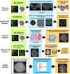
Fig 2. Displaying all the 3D segmentation pipelines together.

The green colored boxes indicate the training process for the respective pipeline. The blue boxes indicate the predicted, semantic segmentations generated by the trained DL algorithms, and the orange boxes indicate phases of postprocessing, leading to the final instance segmentation. The MARS pipeline doesn’t include a training or postprocessing step, but parameter tuning is required. 3D, three-dimensional.

Fig 3. Schematic workflow of the benchmarking process.

The evaluation of segmentation pipelines begins with the training of the DL models on a common training dataset (confocal images and ground truth). The training and postprocessing steps for each pipeline are reproduced in the exact way as defined in the respective papers or their repositories. Then, the 5 pipelines are tested on a common test set of images. The test dataset (Fig 4) contains both raw confocal images and their corresponding expert annotated ground truths, and, therefore, it is possible to assess the segmentation accuracy of the 5 pipelines by comparing segmentation output of each pipeline with the respective ground truth data. Finally, the relative accuracy of each method is evaluated using multiple strategies. DL, deep learning.

Fig 4

(A) The 2 test datasets containing a total of 10 confocal image stacks of 2 different Arabidopsis floral meristems. (B) A sample test stack (TS1-00H) and its segmentation by 5 segmentation pipelines.

Fig 5

(A) Results of VJI metric from the 5 segmentation pipelines. Note that VJI is computed for each pair of segmented image/ ground truth image, and so the VJI statistics shown above are computed on the values of VJI of the 10 3D test images for each pipeline. (B) and (C) shows rates of over- and undersegmentation, which is computed using a segmented stack and corresponding ground truth stack as input. The distributions shown here are estimated over the results from the 2 test datasets TS1 and TS2. (D) Example segmentation results by 5 pipelines on a test image slice. 3D, three-dimensional; VJI, volume-averaged Jaccard index.

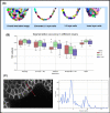
Fig 6

(A) Extracting L1, L2, and inner layers from an input segmented meristem image. (B) Estimating segmentation accuracy (VJI) for different cell layers. All stacks from the test dataset are used for this evaluation. (C) Boundary Intensities profile plot for outer and inner layer cells. The gray value at x = 0 on the plot on the left is the gray value of the image at the red point of the line segment drawn on the right image.

Fig 7

(A) A test image after applying Gaussian noise (var 0.04, 0.08). (B) Variation of segmentation accuracy (VJI) with 3 Gaussian noise variances. (C) Variation in rates of oversegmentation. (D) Variation in rates of undersegmentation. Note that for noise variance of 0.08, Cellpose is unable to identify cells. (E) Example results from the 5 pipelines under the impact of image noise (Gaussian noise variance 0.08). PSNR, peak signal-to-noise ratio; VJI, volume-averaged Jaccard index.

Fig 8

(A) Effect of blurring on an image. (B) Comparing segmentation accuracies of pipelines under the effect of image blur. (C) Comparing rates of oversegmentation. (D) Undersegmentations due to image blur. (E) Results from the 5 pipelines under the impact of image blur.

Fig 9. Impact of image exposure levels on segmentation quality of 5 pipelines.

(A) Examples of partial over- and underexposure. In (B), the VJI values for over- and underexposure are plotted together with the original VJI values for unmodified stacks. Similarly in (C) and (D), the rates of over- and undersegmentation are plotted for the impacts of over- and underexposure alongside those for the unmodified stacks. VJI, volume-averaged Jaccard index.

Fig 10

(A) Sample results from the 5 pipelines under the impact of image overexposure. (B) Results from the 5 pipelines under the impact of partial underexposure.

Fig 11

Slice view of a sample (A) Ascidian embryo image and its (B) ground truth segmentation. (C) Ascidian embryo image (PM03), ground truth, and segmentations by 5 pipelines. (D) VJI values for segmentation results using Ascidian PM data and 5 pipelines. PM, Phallusia mammillata; VJI, volume-averaged Jaccard index.

Fig 12

(A) Ovule image and ground truth along with segmentations by 5 pipelines. (B) VJI values for segmentation results using ovule data and 5 pipelines.

Fig 13

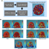
(A) Process to view segmentation quality in 3D on Morphonet.Segmentation quality results (VJI values) for a test stack (TS2-26h) from 5 pipelines displayed on Morphonet. Users can slice through each 3D stack in XYZ directions and check the property (here VJI values) for each cell in the interior layers of the tissue structure. For example, for each pipeline in the above figure, the left image shows the full 3D stack, and the right image shows the cross section of the same stack after slicing 50% in the Z direction. VJI values are projected as a “property” or color map on the cells. In this figure, a “jet” color map is used where red represents high, and blue represents low VJI values as shown in the color bars alongside.3D, three-dimensional; VJI, volume-averaged Jaccard index.

Fig 14. A confocal image is made up by scanning through each point on a 2D plane of an object.

The 3D confocal image is made up of such 2D frames stacked along the Z-axis. Using the 2D Z slices, a full 3D view of the object can be reconstructed. 2D, two-dimensional; 3D, two-dimensional.

Fig 15

(A) Three-dimensional projection of 2 training images and (B) corresponding ground truth segmentations. (C) Lateral (XY) and axial slices (XZ and YZ) of a sample confocal training image.

Fig 16

Plantseg workflow. (A) Input image. (B) Boundary prediction. (C) Final segmentation.

Fig 17. Three-dimensional UNet+ WS workflow.

(A) An input confocal image (xy slice). (B) Class 0 prediction—centroids. (C) Class 1 prediction—background. (D) Class 2 outputcell membranes. (E) An input confocal image (xy slice). (F) Seed image slice. (G) Final segmented slice using watershed on (F).

Fig 18. MRCNN+Watershed workflow.

(A) Creation of instance masks for training MRCNN. (B) Example confocal slice. (C) Two-dimensional predictions by MRCNN. (D) Binary seed image created from identified cell regions in (C). (E) Same slice after 3D segmentation using watershed on the binary seed image. 3D, three-dimensional.

Fig 19. Loss versus epoch plots for training the models from 4 pipelines.

Fig 20

(A) Original ovule image. (B) Impact of using hmin = 2 and sigma value = 0.8 for MARS. (C) Result of MARS on the same image after tuning parameters.

Fig 21

Segmentation quality metric [52] applied to outputs from 5 segmentation pipelines and types of errors displayed as a color map (on a common Z slice). The green cell regions represent regions of complete overlap between ground truth and predicted segmentations (i.e., regions of fully correct segmentation). Red regions represent over and blue regions represent undersegmentation errors. White regions are regions where cells were mistaken for background. The benefit of this metric is that it helps to estimate the rate of over- and undersegmentations as a volumetric statistics and as spatial distributions.

Fig 22. Kernel used for simulating the blur effect on confocal images.

Fig 23

Modification of image intensity (inside selected area within the yellow box). (A) Image intensity transition under partial overexposure. (B) Image intensity variations due to imposition of underexposure.

References

1. Thomas RM, John J. A review on cell detection and segmentation in microscopic images. 2017 International Conference on Circuit, Power and Computing Technologies (ICCPCT). IEEE. 2017:1–5. doi: 10.1109/ICCPCT.2017.8074189 - DOI
1. Hafiz AM, Bhat GM. A survey on instance segmentation: state of the art. Int J Multimed Inf Retr. 2020;9:171–89. doi: 10.1007/s13735-020-00195-x - DOI
1. Vicar T, Balvan J, Jaros J, Jug F, Kolar R, Masarik M, et al.. Cell segmentation methods for label-free contrast microscopy: review and comprehensive comparison. BMC Bioinformatics. 2019;20:360. doi: 10.1186/s12859-019-2880-8 - DOI - PMC - PubMed
1. Lei T, Wang R, Wan Y, Du X, Meng H, Nandi A. Medical Image Segmentation Using Deep Learning: A Survey. arXiv. 2020;abs/2009.13120.
1. Vu QD, Graham S, Kurc T, To MNN, Shaban M, Qaiser T, et al.. Methods for segmentation and classification of digital microscopy tissue images. Front Bioeng Biotechnol. 2019;7:53. doi: 10.3389/fbioe.2019.00053 - DOI - PMC - PubMed
Publication types