A novel computational strategy for defining the minimal protein molecular surface representation

Abstract

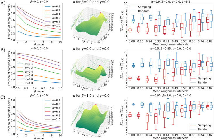
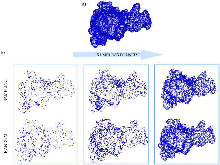
Most proteins perform their biological function by interacting with one or more molecular partners. In this respect, characterizing local features of the molecular surface, that can potentially be involved in the interaction with other molecules, represents a step forward in the investigation of the mechanisms of recognition and binding between molecules. Predictive methods often rely on extensive samplings of molecular patches with the aim to identify hot spots on the surface. In this framework, analysis of large proteins and/or many molecular dynamics frames is often unfeasible due to the high computational cost. Thus, finding optimal ways to reduce the number of points to be sampled maintaining the biological information (including the surface shape) carried by the molecular surface is pivotal. In this perspective, we here present a new theoretical and computational algorithm with the aim of defining a set of molecular surfaces composed of points not uniformly distributed in space, in such a way as to maximize the information of the overall shape of the molecule by minimizing the number of total points. We test our procedure's ability in recognizing hot-spots by describing the local shape properties of portions of molecular surfaces through a recently developed method based on the formalism of 2D Zernike polynomials. The results of this work show the ability of the proposed algorithm to preserve the key information of the molecular surface using a reduced number of points compared to the complete surface, where all points of the surface are used for the description. In fact, the methodology shows a significant gain of the information stored in the sampling procedure compared to uniform random sampling.

Fig 1. Local roughness of the patches.

A) Discretized representation of a molecular surface of the TDP-43 fragment 209-269 (PDB id: 4BS2). Each point of the surface is coloured according to the local roughness value, ${\mathcal{R}}_i$. B) Distribution of the roughness ${\mathcal{R}}_i$ found for each point i of the considered surface.

Fig 2. Sampled points fractions for varying parameters.

Percentage of surface points that are sampled by varying α, β, γ and δ. These plots were obtained after the sampling of the surface of A1.

Fig 3. Analysis of the limit cases of the sampling function.

A) Results obtained when there is no dependency on ${\mathcal{R}}_i$. B) Results obtained when there is no dependency on the distance from the patch center. C) Results obtained with the steepest sampling function. The first column shows the percentage of surface points that are sampled for varying parameters. The second one depicts d for varying parameters; these plots are obtained with an interpolation of the effectively computed values, that -when not set to zero or one- are all the combinations of α = [0.1, 0.2, 0.4, 0.6, 0.8, 1], β = [0, 0.2, 0.4, 0.6, 0.8, 1], γ = [0, 2, 4, 6, 8, 10] and δ = [0, 2, 4, 6, 8, 10]. The last column shows, for the best parameters combination in each limit case, the box plot for different mean ${\mathcal{R}}_i$ of $Z_{t-S}^R$ (in red) and $Z_{t-R}^R$ (in blue). These plots refer again to the application of this sampling method to the surface of A1.

Fig 4. Selection of the absolute best sampling parameters.

A) d as a function of varying values of γ and δ. Each plot is obtained with a fixed value for β, and for all the plots the same fixed value of α = 1.0 is used. The colouring is given by the d value. The plotted surfaces are obtained with an interpolation of the effectively computed values, that were obtained with all the possible combination, for each β value, of γ = [0, 2, 4, 6, 8, 10] and δ = [0, 2, 4, 6, 8, 10]. B) For each plot on the left, the point corresponding to the highest d is selected. The colouring is given by the β value (as described by the color-bar). The plotted surface is obtained from the interpolation of these points, and shows, for all the δ-γ combinations the value of β that will result in the best sampling. The maximum of this surface (red points) corresponds to the best sampling parameters.

Fig 5. Comparison between the best sampling and the random selection of points for patches with different roughness.

A) On the left, an example of how a rough patch is represented with all the points in the surface (whole patch), with only the points resulting from the sampling (sampled points) and with randomly extracted points (random points). On the right, the same three representation cases for a plane patch. B) In red, the box plot for different ranges of patches’ roughness of $Z_{t-S}^R$. In blue, the box plot for different ranges of patches’ roughness of $Z_{t-R}^R$. This is in the case of a sampling with parameters α = 1, β = 0, γ = 6 and δ = 0, whose combination results in the highest value of d for the A1 surface.

Fig 6. Visualization of the 3D surfaces reconstruction.

A) 3D reconstruction of the A1 surface from all its surface points. B) The three columns depict the reconstruction of the same surface, with an increasing sampling density. In each column, the first row shows the reconstruction with a subset of the original points selected with the sampling, whereas the second row shows the reconstruction with a subset that counts the same number of points selected with the sampling, but in this case randomly extracted.

Fig 7. Principal component analysis of the total and sampled points Zernike vectors for four binding regions.

For each of the four considered proteins, the PCA of the Zernike vectors describing the interacting region is performed. The first column shows the projection on the first two PCs of the Zernike vectors of each point in the patch (in blue) and of the points selected with the optimal sampling (in red), with the respective marginal density distributions. The percentage of sampled over total points is reported in the legend. The bar plots in the second column show the percentage of points sampled with different sets of parameters; the bar in the box corresponds to the optimal set. In the third column the percentage of spanned PCs space as a function of the number of sampled points for different sets of parameters is shown. The last column reports the points in the PCs space colored according to the roughness of the centered patch.

References

1. Keskin O, Gursoy A, Ma B, Nussinov R. Principles of protein- protein interactions: what are the preferred ways for proteins to interact? Chemical reviews. 2008;108(4):1225–1244. doi: 10.1021/cr040409x - DOI - PubMed
1. Nooren IM, Thornton JM. Structural characterisation and functional significance of transient protein–protein interactions. Journal of molecular biology. 2003;325(5):991–1018. doi: 10.1016/S0022-2836(02)01281-0 - DOI - PubMed
1. Perkins JR, Diboun I, Dessailly BH, Lees JG, Orengo C. Transient protein-protein interactions: structural, functional, and network properties. Structure. 2010;18(10):1233–1243. doi: 10.1016/j.str.2010.08.007 - DOI - PubMed
1. Berggård T, Linse S, James P. Methods for the detection and analysis of protein–protein interactions. Proteomics. 2007;7(16):2833–2842. doi: 10.1002/pmic.200700131 - DOI - PubMed
1. Vangone A, Bonvin AM. Contacts-based prediction of binding affinity in protein–protein complexes. elife. 2015;4:e07454. doi: 10.7554/eLife.07454 - DOI - PMC - PubMed
Publication types