Towards a safe and efficient clinical implementation of machine learning in radiation oncology by exploring model interpretability, explainability and data-model dependency

Abstract

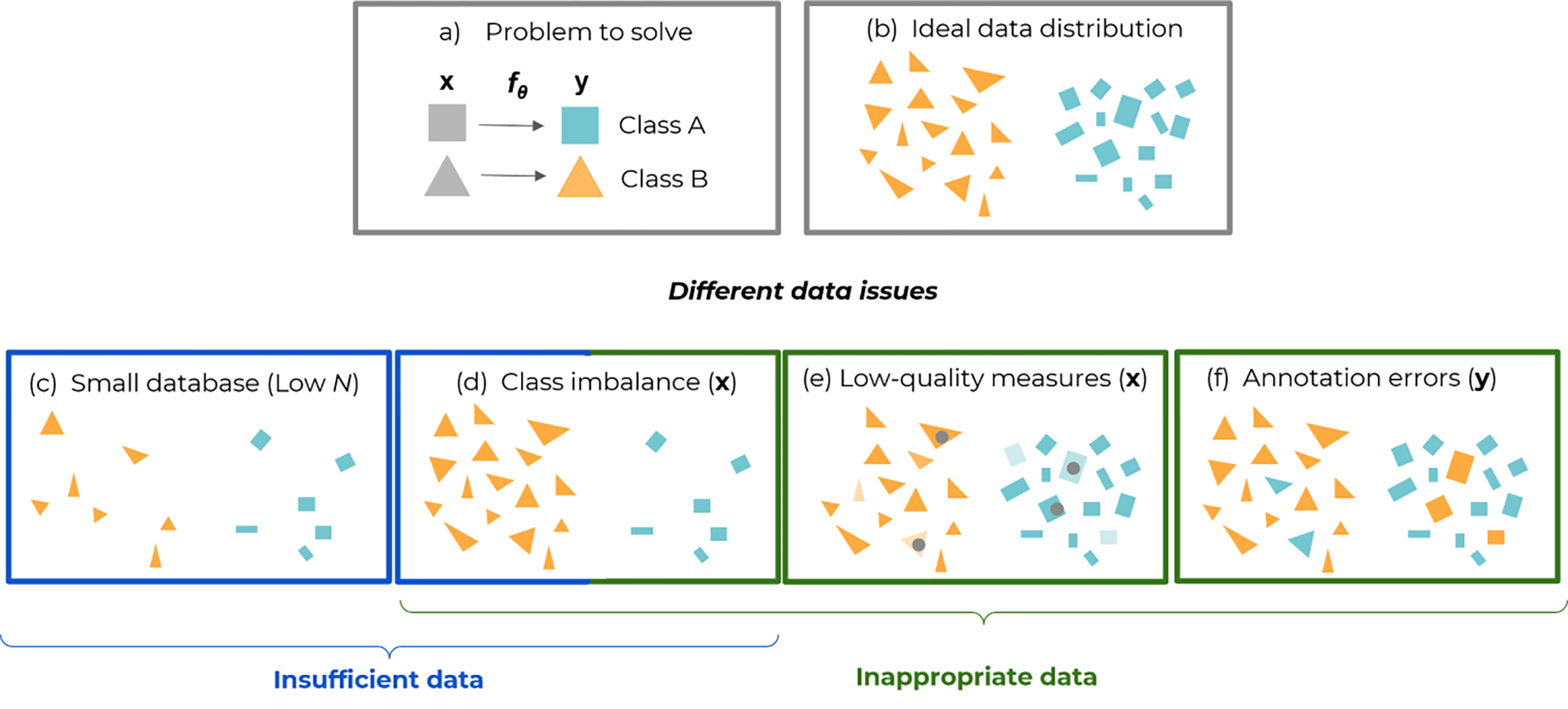
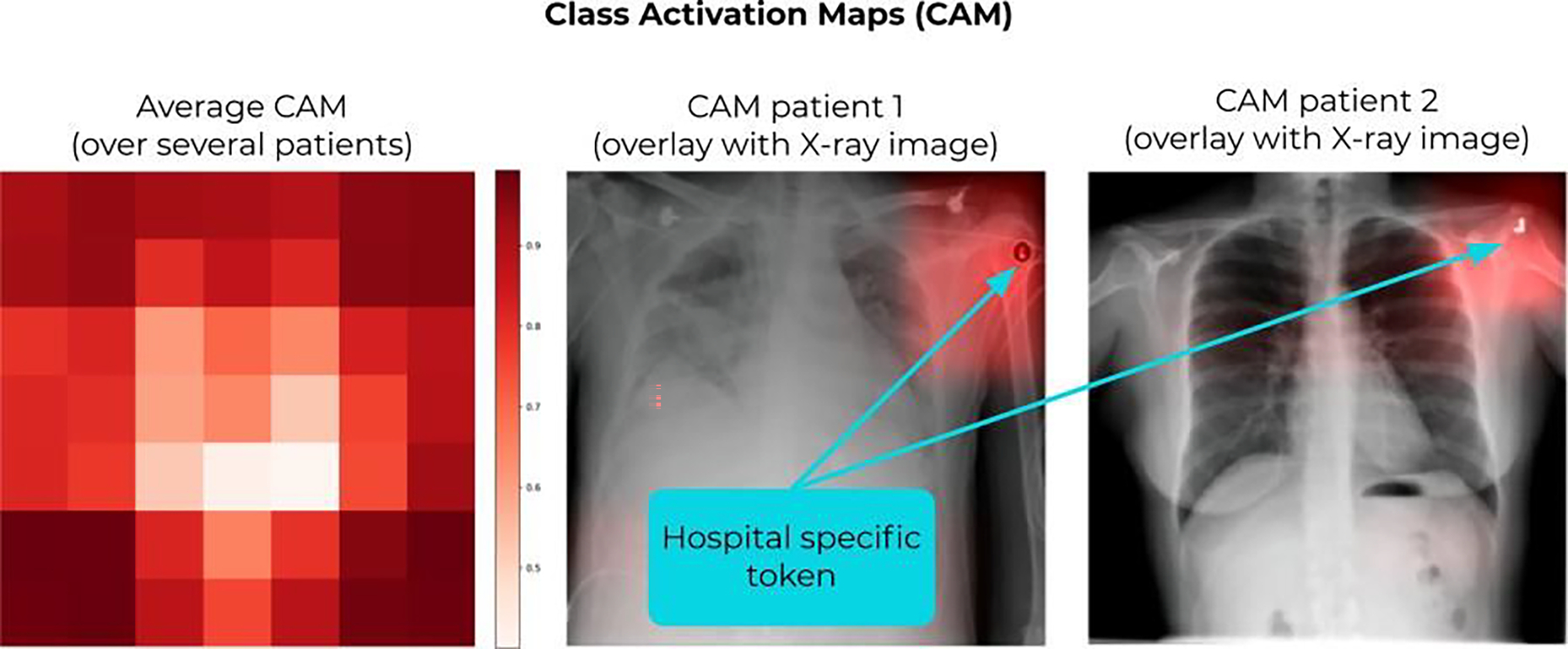
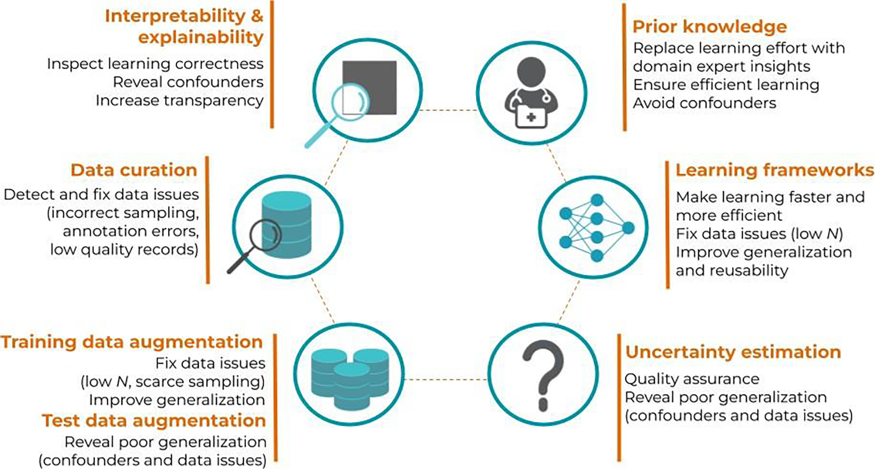
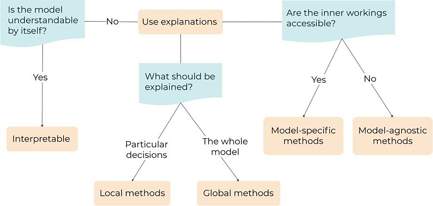
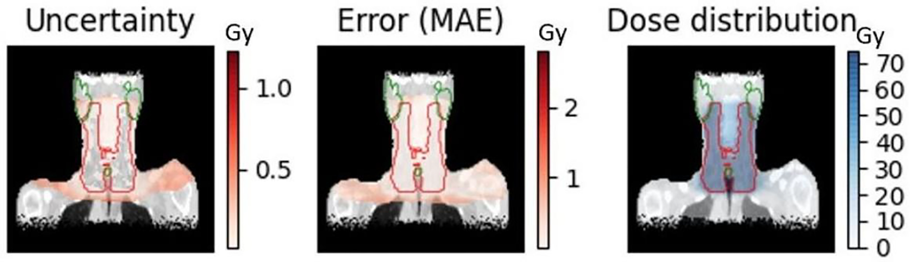
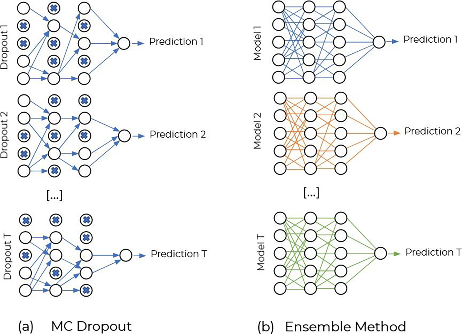
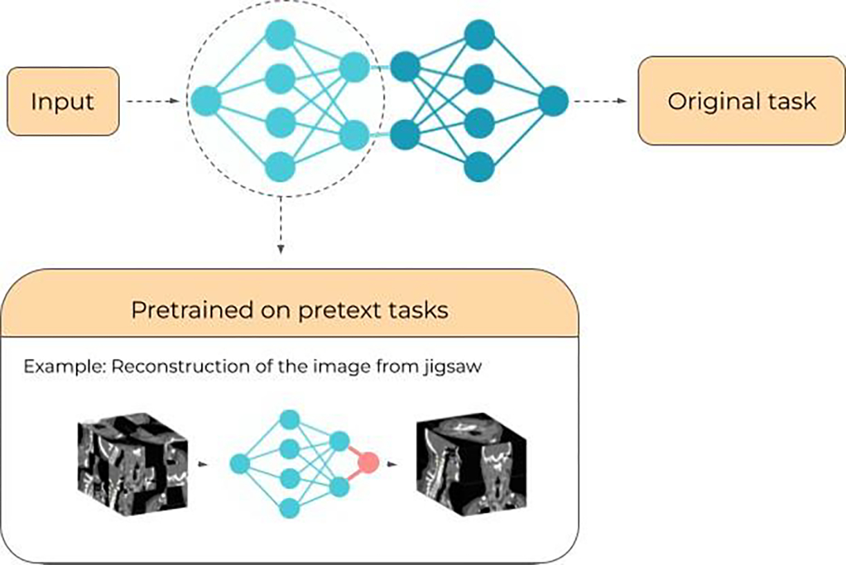
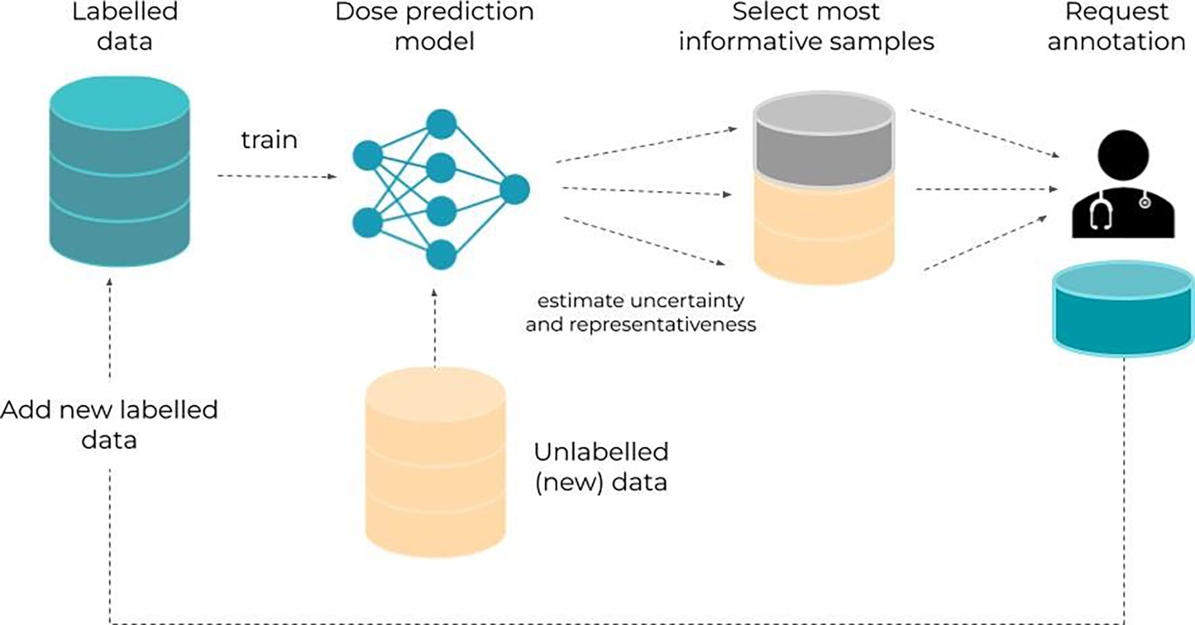
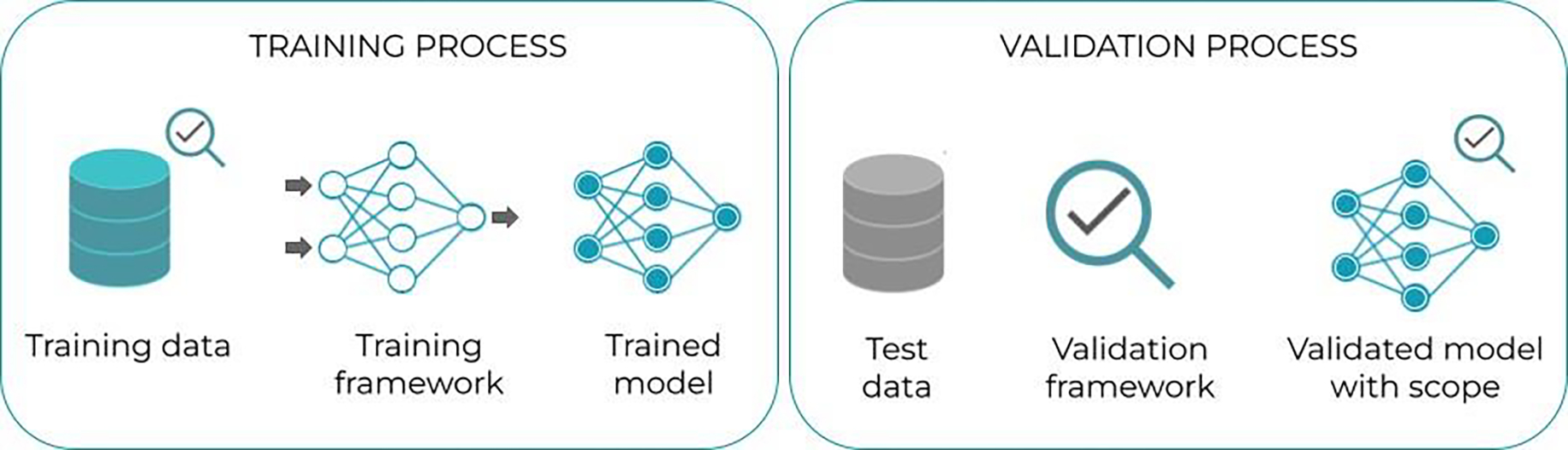
The interest in machine learning (ML) has grown tremendously in recent years, partly due to the performance leap that occurred with new techniques of deep learning, convolutional neural networks for images, increased computational power, and wider availability of large datasets. Most fields of medicine follow that popular trend and, notably, radiation oncology is one of those that are at the forefront, with already a long tradition in using digital images and fully computerized workflows. ML models are driven by data, and in contrast with many statistical or physical models, they can be very large and complex, with countless generic parameters. This inevitably raises two questions, namely, the tight dependence between the models and the datasets that feed them, and the interpretability of the models, which scales with its complexity. Any problems in the data used to train the model will be later reflected in their performance. This, together with the low interpretability of ML models, makes their implementation into the clinical workflow particularly difficult. Building tools for risk assessment and quality assurance of ML models must involve then two main points: interpretability and data-model dependency. After a joint introduction of both radiation oncology and ML, this paper reviews the main risks and current solutions when applying the latter to workflows in the former. Risks associated with data and models, as well as their interaction, are detailed. Next, the core concepts of interpretability, explainability, and data-model dependency are formally defined and illustrated with examples. Afterwards, a broad discussion goes through key applications of ML in workflows of radiation oncology as well as vendors' perspectives for the clinical implementation of ML.

Keywords: clinical implementation; interpretability and explainability; machine learning; radiation oncology; uncertainty quantification.

Figure 1.

Some data-related pitfalls of supervised learning, exemplified with a binary classification problem. Panel (a) formalizes the problem and how the model maps the inputs (features or images) to the outputs (class labels green and orange). Panel (b) shows an ideal dataset with enough data globally (high N) and in each class. Panel (c) illustrates insufficient data, when the number of total examples N is too low (for all classes). Panels (d) to (f) illustrate cases of inappropriate data: (d) Class imbalance, when class populations are unequal and minor classes might not be given enough importance in the performance figures. (e) Low-quality or corrupted inputs x, e.g., blurred, noisy, or artifacted images, represented by a lighter color and gray dots in the figure. (f) Annotation errors (mistakes in class labels y). To some extent, class imbalance can be seen as a particular case of insufficient data, when one of the classes has a low N with respect to the other(s).

Figure 2.

Adapted from (Zech et al 2018). Class activation maps (CAM) showing the relevant regions considered by the CNN to make the prediction. The model in this study was trained to predict pneumonia from X-ray images. By looking at the CAMs, they found out that the model was looking at the corner of the images, and in particular, at the hospital-specific metal token (a hidden confounder) to make the prediction. (Left) CAM averaged over several patients; (middle and right) examples of CAMs for two patients.

Figure 3.

Schematic view of the different concepts presented in this topical review and how they can serve as key solutions to overcome the limitations of current ML models, ultimately ensuring a safe and efficient clinical implementation.

Figure 4.

Pipeline describing the typology and the selection of the explanation method. First, if the model is already understandable, it is said to be interpretable. Second, if the model is not understandable, two questions need to be answered to select the right explanation technique: (1) are the inner workings of the model accessible? and (2) what needs to be explained (the whole model or particular decisions)?

Figure 5.

Inspired by (Ribeiro et al 2016). Workflow illustrating the use of LIME (Local Interpretable Model-agnostic Explanations). The idea of LIME is to learn an interpretable model (e.g., a linear model) to explain individual predictions. In the example, a black box model receives a set of variables for a new patient (i.e. age, smoker, …) and classifies the patient as having lung cancer. The LIME model then provides the user with information (i.e. explanations) about the features that most contributed to the prediction. “Age” and “Sex” did not contribute at all, “Smoker” and “Weight-loss” were against it, while “PET-SUV”, “Histology”, and “Coughing” contributed for the positive lung cancer classification.

Figure 6.

Multi-modal data can be processed in different ways in ML models, depending on how the various modalities are merged. Early fusion (left) is possible if the data types or modalities are not too different. A typical example is given by stacking multiple registered image modalities like CT, MR, PET, which are processed in convolutional layers. Joint fusion (middle) is typical of image data accompanied by simple indicators in vectors or text; then, convolutional layers (model 1) process the images to transform into feature vectors that are then merged (concatenated) with the other indicators to form a longer feature vector to be processed by the final model. Late fusion (right) pushes joint fusion even further: the output is a very simple combination of data coming from separate models dedicated to each data type; to some extent, late fusion bears some similarity with ensemble learning.

Figure 7.

The fundamental difference between a regular neural network (a) and its Bayesian extension (b), holds in the replacement of scalar values (pointwise estimates) with full-fletched probability distributions with an expected value (equivalent to the pointwise estimate) and a standard deviation, indicative of its associated uncertainty. Dealing with probability distributions is much more demanding computationally and several approximations or surrogates to Bayesian networks exist, like neuron dropout in figure 8 and figure 10.

Figure 8.

(a) Standard Neural network where all weights are set. (b) A random fraction of the weights are switched off.

Figure 9.

Prediction uncertainty, prediction error and predicted dose distribution for the same slice of a patient with head and neck cancer (Vanginderdeuren et al 2021).

Figure 10.

(a) MC Dropout at inference time. The T predictions are obtained from Dropout of different weights. (b) Ensemble method, different models have been previously trained and the T predictions are obtained from each network on the same sample.

Figure 11.

Self-supervised learning workflow with an example of a pretext task where the input is the image from which patches have been mixed up. The aim of this pretext task is to reconstruct the initial image hoping the encoder extracts useful features from the data (Inspired from (Taleb et al 2020). The knowledge acquired by the trained network on the pretext task is later used to carry out the main, original task.

Figure 12.

Active learning workflow: unlabelled data gets selected for expert annotation according to the chosen informativeness metric and then added to the training set of the network.

Figure 13.

(a) Traditional Machine Learning where to train a model for a new task, we need a large dataset for the training. (b) Transfer Learning, where knowledge is transferred from another network performing a similar task. The advantage is that the required size of Dataset 2 can be reduced significantly.

Figure 14.

Tentative mapping between common issues that are encountered in the implementation and deployment of machine learning and some possible solutions to overcome them. Since machine learning relies on data-driven models, both the issues and solutions can be seen from the angles of data, modeling, or learning.

Figure 15.

Typical workflow of radiotherapy treatment planning and delivery (top panels, orange boxes) and current applications of ML in the workflow (bottom, blue boxes).

Figure 16.

For the different slices of four patients, the red line corresponds to the clinical contour, the blue to the prediction and the yellow area the 95% confidence band. The latter can be used as a visual indicator of the model uncertainty. For instance the model is more uncertain for patient four (Balagopal et al 2021).

Figure 17.

Model development process.

Figure 18.

Example of data sheet for a released ML model for automatic planning of radiotherapy treatments for prostate cancer patients. The data sheet contains relevant information about the ML model, including the general overview and scope, as well as information about the training and validation phases. This data sheet should be provided by the vendor together with the model.

Figure 19.

Commissioning and go-live for a released ML model.

References

1. Abdar M, Pourpanah F, Hussain S, Rezazadegan D, Liu L, Ghavamzadeh M, Fieguth P, Cao X, Khosravi A, Rajendra Acharya U, Makarenkov V and Nahavandi S 2021. A review of uncertainty quantification in deep learning: Techniques, applications and challenges Information Fusion 76 243–97 Online: 10.1016/j.inffus.2021.05.008 - DOI
1. Adadi A and Berrada M 2018. Peeking Inside the Black-Box: A Survey on Explainable Artificial Intelligence (XAI) IEEE Access 6 52138–60 Online: 10.1109/access.2018.2870052 - DOI
1. Afshar P, Mohammadi A, Plataniotis KN, Oikonomou A and Benali H 2019. From Handcrafted to Deep-Learning-Based Cancer Radiomics: Challenges and Opportunities IEEE Signal Processing Magazine 36 132–60 Online: 10.1109/msp.2019.2900993 - DOI - PMC - PubMed
1. Ahishakiye E, Van Gijzen M B, Tumwiine J, Wario R and Obungoloch J 2021. A survey on deep learning in medical image reconstruction Intelligent Medicine 1 118–27 Online: 10.1016/j.imed.2021.03.003 - DOI
1. Ahn SH, Kim E, Kim C, Cheon W, Kim M, Lee SB, Lim YK, Kim H, Shin D, Kim DY and Jeong JH 2021. Deep learning method for prediction of patient-specific dose distribution in breast cancer Radiat. Oncol. 16 154. - PMC - PubMed
Publication types