. 2022 Apr 19;13(1):2116.
doi: 10.1038/s41467-022-29677-8.

A decade of cold Eurasian winters reconstructed for the early 19th century

Affiliations

A decade of cold Eurasian winters reconstructed for the early 19th century

Lukas Reichen et al. Nat Commun. .

Abstract

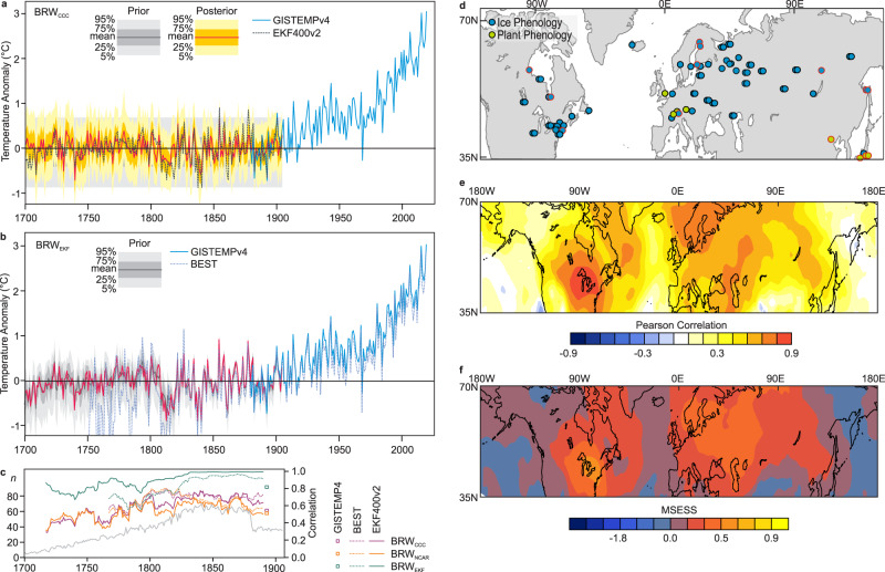
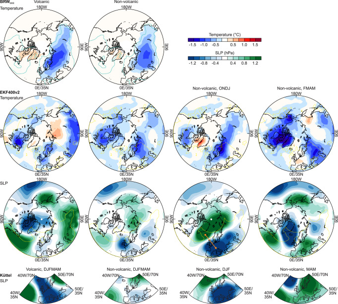
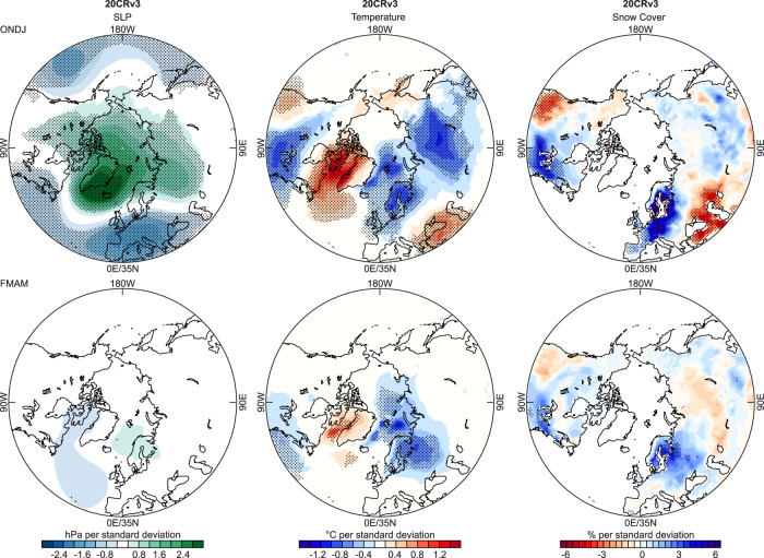
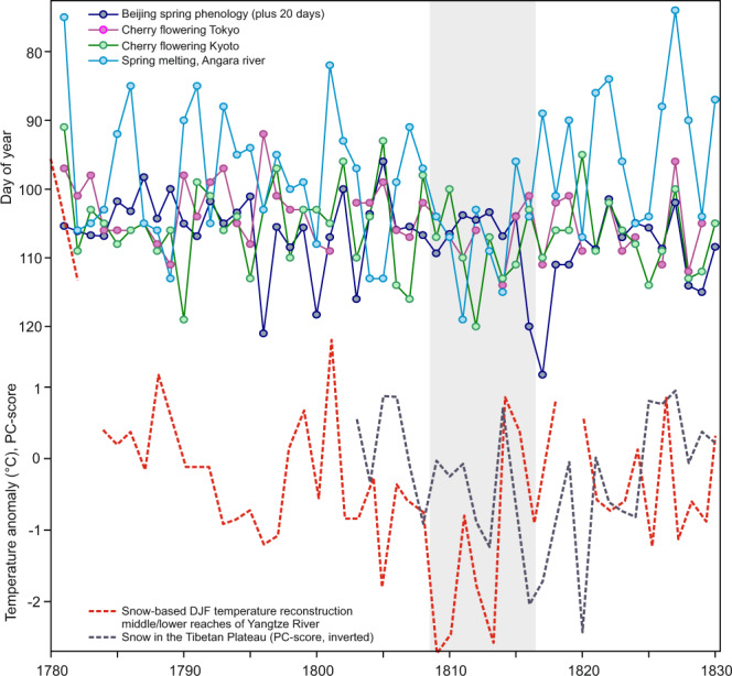
Annual-to-decadal variability in northern midlatitude temperature is dominated by the cold season. However, climate field reconstructions are often based on tree rings that represent the growing season. Here we present cold-season (October-to-May average) temperature field reconstructions for the northern midlatitudes, 1701-1905, based on extensive phenological data (freezing and thawing dates of rivers, plant observations). Northern midlatitude land temperatures exceeded the variability range of the 18th and 19th centuries by the 1940s, to which recent warming has added another 1.5 °C. A sequences of cold winters 1808/9-1815/6 can be explained by two volcanic eruptions and unusual atmospheric flow. Weak southwesterlies over Western Europe in early winter caused low Eurasian temperatures, which persisted into spring even though the flow pattern did not. Twentieth century data and model simulations confirm this persistence and point to increased snow cover as a cause, consistent with sparse information on Eurasian snow in the early 19th century.


Conflict of interest statement

The authors declare no competing interests.

Figures

Fig. 1
Fig. 1. Cold-season temperatures from 1701 to 2020 over northern midlatitude land areas.
a, b Time series of cold-season temperatures over land areas between 35 and 70°N from BRWCCC and BRWEKF (including prior and posterior; not shown for BRWEKF for better visualisation) as well as BEST, and GISTEMP4. Anomalies are relative to the period of overlap (1880–1905). c 31-yr moving correlations between our reconstructions and other time series (only 25 years of overlap are available for GISTEMP4). The number of assimilated observations n is shown in grey. d Locations of the 68 phenological series that entered the reconstruction (black circles) and the 14 used for evaluation (red circles). Pearson correlation (e) and mean-squared error skill score (MSESS, f) of BRWCCC evaluated against EKF400v2, 1851–1900.
Fig. 2
Fig. 2. Cold-season temperature anomalies (with respect to 1851–1900) during the cold spell in the early 19th century in different reconstructions.
Anomalies in 1808/9–1815/6 in BRWCCC, BRWNCAR, ANACCC, ANANCAR, BRWEKF, and EKF400v2. Dashed (−1) and solid (+1) red lines express anomalies in standard deviations of the 1851–1900 period. The green dashed lines indicate a MSESS of 0.2 relative to EKF400v2 (the yellow dashed line in EKF400 indicates an MSESS of 0.2 relative to HadCRUT5, which is not spatially complete).
Fig. 3
Fig. 3. Volcanic effects and internal variability.
Temperature and SLP anomalies (with respect to 1851–1900) in (left) the two cold seasons following volcanic eruptions and (second from left) the remaining 6 years of the period in BRWCCC and EKF400v2. For the latter composite, anomalies are also shown for Oct-Jan and Feb-May separately. For SLP we also show composites from Küttel et al. for Dec-May, Dec-Feb, and Mar-May. The green lines indicate a MSESS of 0.2 relative to EKF400 (the yellow dashed line in EKF400 indicates an MSESS of 0.2 relative to HadCRUT5 and HadSLP2). The thick orange line illustrates the index defined.
Fig. 4
Fig. 4. Seasonal persistence.
Standardised regression coefficients of detrended SLP, temperature, and snow cover in Oct-Jan (top) and Feb-May (bottom) onto a detrended Oct-Jan SLP index (defined as the difference between two points, indicated in Fig. 3) in 20CRv3, 1901–2000. Significant (p < 0.05) coefficients are hatched.
Fig. 5
Fig. 5. Day-of-year (note the reverse scale) of spring phenological dates from East Asia (Table S1) as well as a winter temperature reconstruction based on documentary snow data and a snow proxy from Tibet (lower scale).
Note that none of these six series was used in BRWCCC, BRWNCAR, and BRWEKF. The grey shading indicates the period of interest.

Similar articles

Cited by

References

    1. Lenssen N, et al. Improvements in the GISTEMP uncertainty model. J. Geophys. Res. Atmos. 2019;124:6307–6326. doi: 10.1029/2018JD029522. - DOI
    1. Osborn TJ, et al. Land surface air temperature variations across the globe updated to 2019: the CRUTEM5 dataset. J. Geophys. Res. 2021;126:e2019JD032352. doi: 10.1029/2019JD032352. - DOI
    1. Rohde, R. et al. A new estimate of the average earth surface land temperature spanning 1753 to 2011. Geoinfor Geostat: An Overview1, 1 (2013).
    1. Shah SK, et al. A winter temperature reconstruction for the Lidder Valley, Kashmir, Northwest Himalaya based on tree-rings of Pinus wallichiana. Clim. Dyn. 2019;53:4059–4075. doi: 10.1007/s00382-019-04773-6. - DOI
    1. Wilson R, et al. Last millennium Northern Hemisphere summer temperatures from tree rings: Part I: the long term context. Quat. Sci. Rev. 2016;134:1–18. doi: 10.1016/j.quascirev.2015.12.005. - DOI

Publication types