Identifying Mobile Sensing Indicators of Stress-Resilience

Abstract

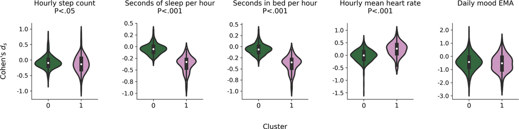
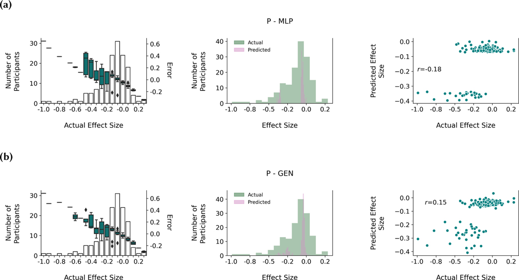
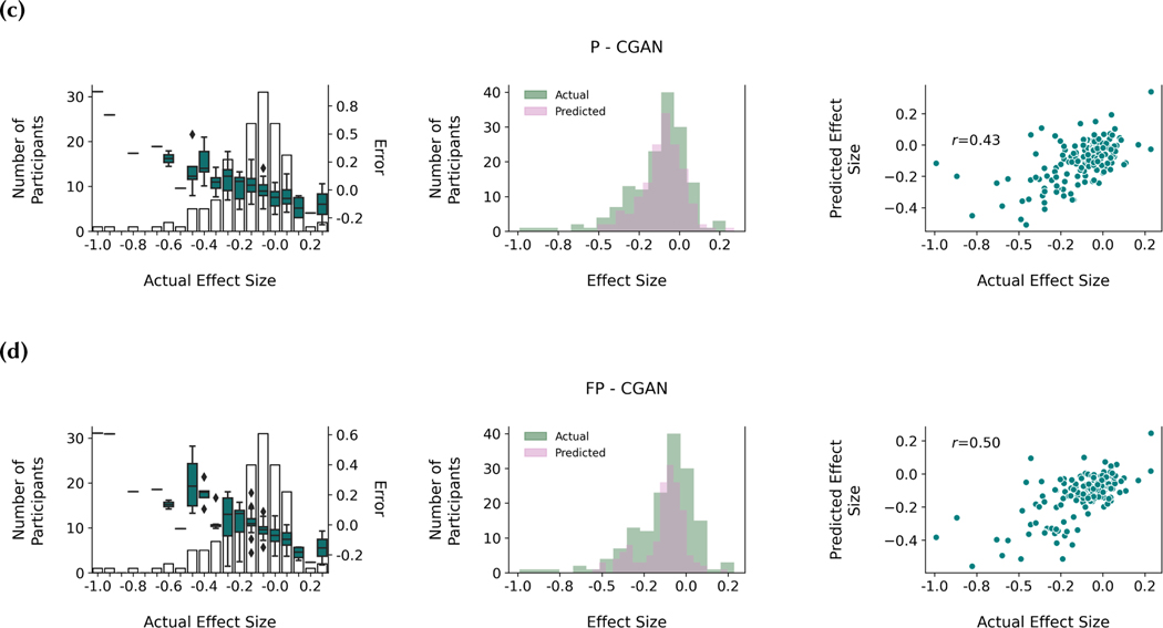
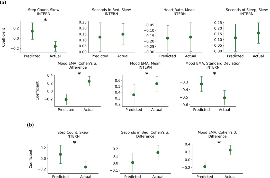
Resident physicians (residents) experiencing prolonged workplace stress are at risk of developing mental health symptoms. Creating novel, unobtrusive measures of resilience would provide an accessible approach to evaluate symptom susceptibility without the perceived stigma of formal mental health assessments. In this work, we created a system to find indicators of resilience using passive wearable sensors and smartphone-delivered ecological momentary assessment (EMA). This system identified indicators of resilience during a medical internship, the high stress first-year of a residency program. We then created density estimation approaches to predict these indicators before mental health changes occurred, and validated whether the predicted indicators were also associated with resilience. Our system identified resilience indicators associated with physical activity (step count), sleeping behavior, reduced heart rate, increased mood, and reduced mood variability. Density estimation models were able to replicate a subset of the associations between sleeping behavior, heart rate, and resilience. To the best of our knowledge, this work provides the first methodology to identify and predict indicators of resilience using passive sensing and EMA. Researchers studying resident mental health can apply this approach to design resilience-building interventions and prevent mental health symptom development.

Keywords: Applied computing → Life and medical sciences; Computing methodologies → Artificial intelligence; Human-centered computing → Empirical studies in ubiquitous and mobile computing; deep generative models; mental health; mobile sensing; wearable technology.

Fig. 1.

Summary of the 37 different indicators used in this work. Values are either specific to the period before (BL), during (INTERN) the internship, or captured a difference in a specific metric between the INTERN and BL periods (Cohen’s d_s). The indicators on the right are calculated for each metric listed in the same section on the left. For example, we calculated the Mean, Standard Deviation, and Skew for both the BL and INTERN periods, as well as the Cohen’s d_s for the mean heart rate. This results in 7 total indicators for the mean heart rate, and this process can be repeated for each of the 5 hourly features (35 indicators). 2 additional indicators were created to capture information about missing data, specifically the count of data per participant in the BL and INTERN periods, resulting in 37 total indicators.

Fig. 2.

The resulting trajectories from the 4-class quadratic growth mixture model. Each curve represents the change in depression symptom trajectory for the subset of the population within that class. Points represent the mean ΔPHQ − 9 (change in depression symptoms) for that period and population subset represented by that trajectory, and error bars are a 95% confidence interval around the mean. The y-axis, ΔPHQ − 9, are the changes in depression symptoms compared to baseline (BL). The x-axis describes the period in which depression symptoms were measured, including the baseline period before the internship (BL), and each quarter, or 3-month period (Q1–4), of the year-long internship. One class was labeled the “Stress-Resilient” class, because it contained a subset of the population who experienced minimal changes in depression symptoms throughout the internship. The legend shows the labels for each class, as well as the size of the population subset (n) the trajectories represent.

Fig. 3.

The full analysis pipeline in this work. We let A be the multivariate hourly baseline (BL) feature distributions per-individual, and B′ be the predicted multivariate hourly internship (INTERN) feature distribution per-individual. (1) We first found relationships between the actual mobile sensing indicators using both the baseline and internship data and resilience (see Table 9). We then built conditional generative adversarial networks (CGANs) to predict the internship data (B′) from the baseline data (A) per-individual. We calculated predicted mobile sensing indicators using both A and B′. Lastly, in (3),we validated whether the associations between the predicted indicators and resilience were equivalent to the relationships between the actual indicators and resilience (see Table 12 and Figure 7).

Fig. 4.

The distribution (histograms) of Cohen’s d_s for training (n = 611) and testing (n = 154) data. Within each histogram, the boxplots show the median and interquartile range (IQR) of each Cohen’s d_s. The numbers below the x-ticks are the IQR of the Cohen’s d_s for the specified dataset.

Fig. 5.

The distribution (histograms) of Cohen’s d_s for the two clusters created for participant multitasking models within the training data. Cluster 0 contained n = 510 participants and cluster 1 contained n = 111 participants. Within each histogram, the boxplots show the median and interquartile range (IQR) of each Cohen’s d_s. The P values listed above each boxplot are the result of either a two-sample t-test or Mann-Whitney U test with the null-hypothesis that the feature distribution centers of each cluster were equal.

Fig. 6.

Comparing test set results across different models for the seconds of sleep per hour feature. (a) shows results for the participant multitasking multilayer perceptron (P - MLP) model, (b) the participant multitasking generator model (P GEN), (c) the participant multitasking conditional generative adversarial network (P - CGAN) model, and (d) the feature and participant multitasking conditional generative adversarial network (FP - CGAN) model. The left column plots show the error (predicted - actual) distributions between the individual-level actual and predicted Cohen’s d_s. The boxplots overlay a histogram describing the number of participants whose actual Cohen’s d_s fell into a designated range. Each box represents the error distribution for the participants within the underlying Cohen’s d_s range. The middle column shows a histogram comparing the actual and predicted Cohen’s d_s, and the right column shows this information in a scatterplot, where each point represents a test individual with the skipped correlation coefficient [103] values (r) labeled.

Fig. 6.

Comparing test set results across different models for the seconds of sleep per hour feature. (a) shows results for the participant multitasking multilayer perceptron (P - MLP) model, (b) the participant multitasking generator model (P GEN), (c) the participant multitasking conditional generative adversarial network (P - CGAN) model, and (d) the feature and participant multitasking conditional generative adversarial network (FP - CGAN) model. The left column plots show the error (predicted - actual) distributions between the individual-level actual and predicted Cohen’s d_s. The boxplots overlay a histogram describing the number of participants whose actual Cohen’s d_s fell into a designated range. Each box represents the error distribution for the participants within the underlying Cohen’s d_s range. The middle column shows a histogram comparing the actual and predicted Cohen’s d_s, and the right column shows this information in a scatterplot, where each point represents a test individual with the skipped correlation coefficient [103] values (r) labeled.

Fig. 7.

Plots of the shared significant coefficients from GEE using calculated features from the actual and predicted data. All features were either calculated using generated data from the internship (INTERN) or a difference between the internship and baseline periods (Difference). (a) shows the coefficient differences from the univariate and (b) from the multivariate GEE. There is a single plot per feature. The y-axis on each plot is the resulting β coefficient from conducting GEE to measure the effect of the feature from distinguishing stress-resilient versus sensitive individuals. The x-axis dictates whether the plotted values are from the GEE using the actual or predicted values. Points are the mean value of the coefficient, and error bars represent 95% confidence intervals. * indicates that the coefficients are significantly (α = 0.05) different.

References

-
- Abadi Martín, Chu Andy, Goodfellow Ian, McMahan H. Brendan, Mironov Ilya, Talwar Kunal, and Zhang Li. 2016. Deep Learning with Differential Privacy. Proceedings of the 2016 ACM SIGSAC Conference on Computer and Communications Security (Oct. 2016), 308–318. 10.1145/2976749.2978318 arXiv: 1607.00133. - DOI
- Adler Daniel A, Ben-Zeev Dror, Tseng Vincent W-S, Kane John M, Brian Rachel, Campbell Andrew T, Hauser Marta, Scherer Emily A, and Choudhury Tanzeem. 2020. Predicting Early Warning Signs of Psychotic Relapse From Passive Sensing Data: An Approach Using Encoder-Decoder Neural Networks. JMIR mHealth and uHealth 8, 8 (Aug. 2020), e19962. 10.2196/19962 - DOI - PMC - PubMed
- Almahairi Amjad, Rajeswar Sai, Sordoni Alessandro, Bachman Philip, and Courville Aaron. 2018. Augmented CycleGAN: Learning Many-to-Many Mappings from Unpaired Data. In Proceedings of the 35th International Conference on Machine Learning (ICML’18). ICML, Stockholm, Sweden. http://arxiv.org/abs/1802.10151 arXiv: 1802.10151.
- American Psychological Association. 2015. 2015 Stress in America Snapshot. https://www.apa.org/news/press/releases/stress/2015/snapshot Library Catalog: www.apa.org.
Grants and funding
LinkOut - more resources
Full Text Sources
Research Materials