Hidden Markov modeling for maximum probability neuron reconstruction

Abstract

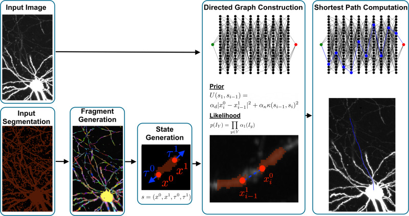
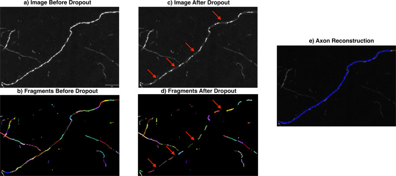
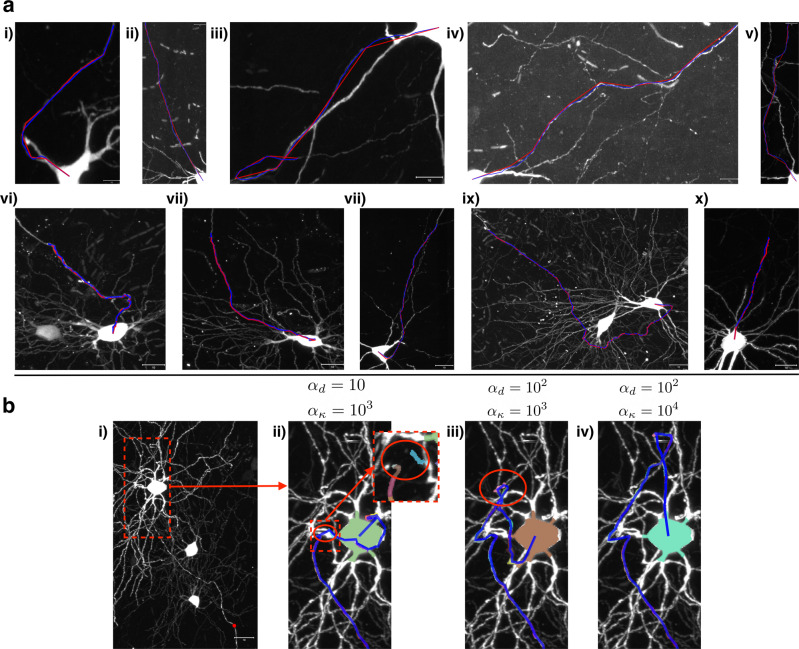
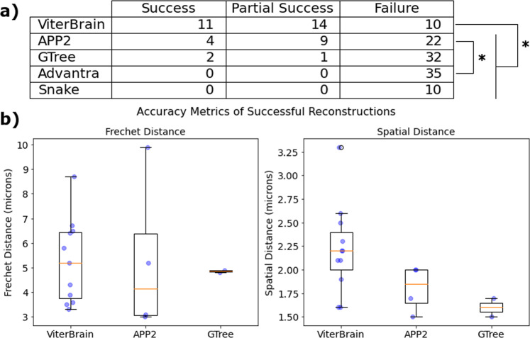
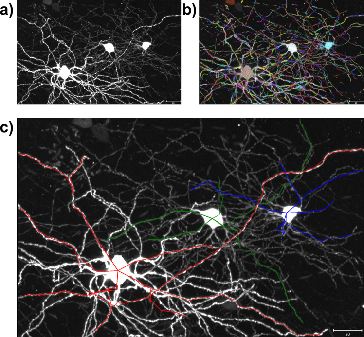
Recent advances in brain clearing and imaging have made it possible to image entire mammalian brains at sub-micron resolution. These images offer the potential to assemble brain-wide atlases of neuron morphology, but manual neuron reconstruction remains a bottleneck. Several automatic reconstruction algorithms exist, but most focus on single neuron images. In this paper, we present a probabilistic reconstruction method, ViterBrain, which combines a hidden Markov state process that encodes neuron geometry with a random field appearance model of neuron fluorescence. ViterBrain utilizes dynamic programming to compute the global maximizer of what we call the most probable neuron path. We applied our algorithm to imperfect image segmentations, and showed that it can follow axons in the presence of noise or nearby neurons. We also provide an interactive framework where users can trace neurons by fixing start and endpoints. ViterBrain is available in our open-source Python package brainlit.

Fig. 1. Image segmentation models sever neuronal processes.

a An image subvolume from the MouseLight project containing a single neuron. b The same image overlaid with a binary image mask in brown. This mask was generated by the random forest based software Ilastik and illustrates the typical output of an image segmentation model. c The same binary image mask, with a different color for each connected component. The variety of colors shows that the neuron has been severed into several pieces. All panels are maximum intensity projections (MIPs), and the scale bar represents 15 microns.

Fig. 2. Summary of the ViterBrain algorithm.

The algorithm takes in an image and a binary mask that might have severed, or fused neuronal processes. First, the mask is processed into a set of fragments. For each fragment, the endpoints (x⁰, x¹) and endpoint orientations (τ⁰, τ¹) are estimated and added to the state space. Next, transition probabilities are computed from both the image and state data to generate a directed graph reminiscent of the trellis graph in classic hidden Markov modeling. The transition prior depends on spatial distance between fragments, $\mid x_i^0-x_{i-1}^1\mid$, and curvature of the path that connects them, κ(s_i−1, s_i), and these two terms are balanced by the hyperparameters α_d, α_κ. The transition likelihood depends on the local image intensity α₁(I_y). Finally, a shortest path algorithm is applied to compute the maximally probable state sequence connecting the start to the end state.

Fig. 3. Characterization of voxel intensity distributions in three different subvolumes of one of the Mouselight whole-brain images.

a Correlation of intensities between voxels at varying distances from each other. The curves show that intensities are only weakly correlated (ρ < 0.4) at a distance of > 10 microns for foreground voxels, or a distance of > 2 microns for background voxels. Error bars represent a single standard deviation of the Fisher z-transformation of the correlation coefficient. Each curve was generated from all pairs of 5000 randomly sampled voxels. b Kernel density estimates (KDEs) of foreground and background intensity distributions. A subset of the voxels in each subvolume was manually labeled, then used to train an Ilastik model to classify the remaining voxels. Each KDE was generated from 5000 voxels, according to the Ilastik classifications. KDEs were computed using scipy’s Gaussian KDE function with default parameters.

Fig. 4. Demonstration of maximally probable reconstruction on isolated linear structures.

a A satellite image of part of the Great Wall of China and b a neuronal process from the MouseLight dataset (MIP). Left panels show the original images. Middle panels shows the space of fragments, $\mathcal{F}$, pictured in color. The green and red arrows indicate the start and end states of the reconstruction task, respectively. The right panels show the most probable fragment sequences, where the fragments are colored and overlaid with a blue line connecting the endpoints of the fragments. The scale bar in b represents 10 microns.

Fig. 5. ViterBrain is robust to image intensity and fragment dropout when axons are relatively isolated.

a An image subvolume from the MouseLight project containing an axon. The scale bar represents 20 microns. b The same image, overlaid with the fragments which are depicted in different colors. c The image intensity was censored periodically along an axon path (red arrows). d The fragments associated with the censored regions were removed from the fragment space (red arrows). e Nonetheless, our algorithm was able to jump over the censored regions to reconstruct this axon. All images are MIPs.

Fig. 6. Demonstration of ViterBrain.

a Successful axon reconstructions; the ViterBrain reconstructions are shown by the blue line; the manual reconstructions are shown by the red line. The algorithm was run with the same hyperparameters in each case: α_d = 10 and α_κ = 1000. b Different hyperparameter values lead to different results. Panel i shows the neuron of interest. Panels ii–iv are close-up views of reconstructions with different hyperparameter values that weigh transition distance (α_d) and transition curvature (α_κ). The red circle in Panel ii indicates where the reconstruction deviated from the true path by jumping ~ 10μm to connect the gray fragment to the light blue fragment. Panel iii shows how a higher α_d value avoids the jump in panel ii, but takes a sharp turn to deviate from the true path (red circle). Finally, in panel iv), the reconstruction avoids both the jump from panel ii) and the sharp turn from panel iii) and follows the true path of the axon back to the cell body. All images are MIPs, and all scale bars represent 10 microns.

Fig. 7. Results of reconstruction algorithms on a dataset of 35 subvolumes of a MouseLight whole brain image.

(Snake was only applied to 10 subvolumes due to incoherent results and excessively slow runtimes, see Fig. S4). Each subvolume contained a soma and part of its axon. The task was to reconstruct the portion of the axon that was contained in the image (no branching). First, the algorithms were evaluated visually and classified as successful, partially successful (over half, but not all, of the axon reconstructed), or failed. The table in panel a shows these results, along with markers showing statistical significance in a two proportion z-test comparing success rates of the algorithms at α = 0.05. For each successful reconstruction, we measured the Frechet distance and spatial distance from the manual ground truth in order to evaluate the precision of the reconstructions. These distances are shown as blue points in b, overlaid with standard box and whisker plots (center line, median; box limits, upper and lower quartiles; whiskers, 1.5x interquartile range; points, outliers).

Fig. 8. Proof of concept graphical user interface.

a Image subvolume presented to the user. b Neuron fragments also shown in different colors. The user can then click on two fragments and generate the most probable curve between them. c Three partial reconstructions (red, green and blue) of different neurons using the GUI. The scale bars represent 20 microns.

References

1. Winnubst J, et al. Reconstruction of 1,000 projection neurons reveals new cell types and organization of long-range connectivity in the mouse brain. Cell. 2019;179:268–281. doi: 10.1016/j.cell.2019.07.042. - DOI - PMC - PubMed
1. Peng, H., Meijering, E. & Ascoli, G. A. From diadem to bigneuron. Springer (2015). - PMC - PubMed
1. Peng H, Ruan Z, Long F, Simpson JH, Myers EW. V3d enables real-time 3d visualization and quantitative analysis of large-scale biological image data sets. Nat. Biotechnol. 2010;28:348–353. doi: 10.1038/nbt.1612. - DOI - PMC - PubMed
1. Acciai L, Soda P, Iannello G. Automated neuron tracing methods: an updated account. Neuroinformatics. 2016;14:353–367. doi: 10.1007/s12021-016-9310-0. - DOI - PubMed
1. Peng H, Ruan Z, Atasoy D, Sternson S. Automatic reconstruction of 3d neuron structures using a graph-augmented deformable model. Bioinformatics. 2010;26:38–46. doi: 10.1093/bioinformatics/btq212. - DOI - PMC - PubMed
Publication types