The importance of warm habitat to the growth regime of cold-water fishes

Abstract

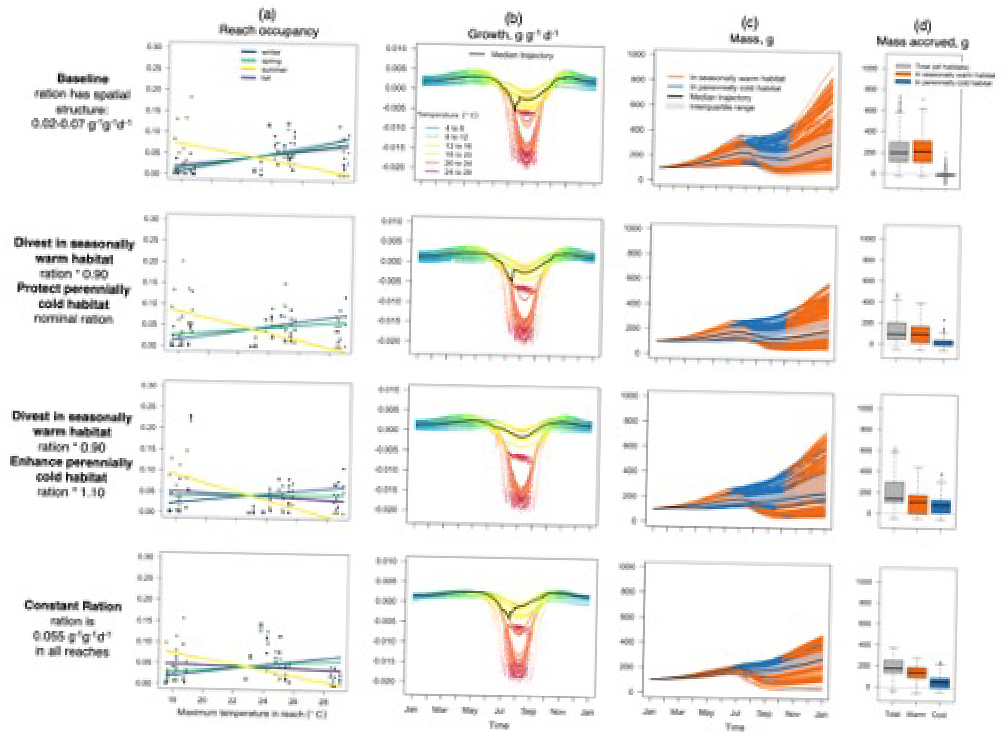
A common goal of biological adaptation planning is to identify and prioritize locations that remain suitably cool during summer. This implicitly devalues areas that are ephemerally warm, even if they are suitable most of the year for mobile animals. Here we develop an alternative conceptual framework, the growth regime, which considers seasonal and landscape variation in physiological performance, focusing on riverine fish. Using temperature models for 14 river basins, we show that growth opportunities propagate up and down river networks on a seasonal basis, and that downstream habitats that are suboptimally warm in summer may actually provide the majority of growth potential expressed annually. We demonstrate with an agent-based simulation that shoulder-season use of warmer downstream habitats can fuel annual fish production. Our work reveals a synergy between cold and warm habitats that could be fundamental for supporting coldwater fisheries, highlighting the risk in conservation strategies that underappreciate warm habitats.

Extended Data Fig. 1

Biweekly changes in the landscape patterning of fish growth potential for the John Day River Basin, Oregon, USA.

Extended Data Fig. 2:

River network used in simulation of fish movement and foraging.

Extended Data Fig. 3

Parameters used in individual-based model.

Extended Data Fig. 4

Sensitivity analysis for simulation model.

Extended Data Fig. 5

Simulation results from the individual-based fish model for each of 4 scenarios.

Figure 1 |. Example of how freshwater climate change adaptation devalues ephemerally warm habitats.

Data are simulated to provide a generic example unless otherwise stated. (a) Spatial stream network models generate maps of present or future August water temperatures (here red is warmer, and blue is colder). (b) Opportunistically compiled datasets of species presence/absence (i.e., occupancy) are plotted against August temperature. The occupancy data are most frequently recorded during summer base flow conditions. (c) Occupancy thresholds (e.g., >80% probability of occurrence) are used to define climate refugia, which are prioritized by climate-smart planning. This framework pervasively devalues downstream or mainstem river habitat (shown in orange here) in favor of tributaries (gray). However, locations that exceed summer temperature thresholds are cool most of the year, as illustrated by time-series of temperature from contrasting sites in a single watershed (Upper Klamath Basin, USA, panels mapped onto example network for illustrative purposes only), and (d) a plot of the proportion of the year that rivers exceed different thresholds for daily mean temperature, based on data for 72 sites in Oregon basins listed as temperature impaired by the United States Environmental Protection Agency.

Figure 2 |. The growth regime of rivers and its implications for mobile fish.

(a) Example of contrasting mainstem and tributary water temperatures from the John Day River, Oregon, USA; (b) A scope for growth curve for a coldwater fish (shaded black where growth is positive), (c) Inputting the time-series of temperature into the growth model yields seasonal patterns of growth potential for headwater and mainstem habitat; (d) cumulative growth potential for a sedentary fish in the mainstem or tributary habitat, or for a mobile fish that couples the two habitat types to maximize growth potential. Ecological conditions determine the extent to which this growth potential is realized in nature. See Methods for full description of analysis.

Figure 3 |. Seasonal variation in the landscape patterning of fish growth potential in the John Day River Basin, Oregon, USA.

Maps show physiological growth potential (grams fish•wk¹) for a coldwater fish (bull trout) based on water temperature. The spatiotemporal data on water temperature are from a published model using remotely sensed land surface temperatures. Physiological growth potential was calculated from a published bioenergetics model parameterized for bull trout. Each map shows resulting growth potential for a single week from each season (the full annual cycle at bi-weekly resolution is shown in extended data fig. 1). Circular barplot in center shows the area of thermally optimal (10–16°C) habitat across the landscape, at weekly resolution. Each weekly bar is divided into the proportion occurring in lower order (1–3) tributary habitat (dark gray), and higher order (4–7) mainstem habitat (light gray). Inset panel shows map of lower order and higher order portions of network.

Figure 4 |. Variation among riverscape growth regimes

(a) left column shows maps and corresponding histograms of the fall-summer growth differential (FSGD, units: grams fish•wk⁻¹) for the Upper Grande Ronde (UGR), Tucannon (TUC), and South Fork Salmon (SFS) river basins. The y-axis of each histogram (omitted for clarity) is the number of stream reaches observed for each FSGD bin. Positive FSGD values indicate bimodal growth regimes and negative, unimodal, as illustrated by inset plot for three contrasting sites from the UGR Basin (y-axis: growth potential in grams fish•wk⁻¹). Right column: (b) the proportion of annual positive growth potential that occurs in seasonally warm reaches, for different basins (x-axis) and years (color). This is the sum of growth potential in reaches where the maximum weekly median temperature is > 17°C, divided by the sum of growth potential across all reaches. (c) Seasonal variation in the area of thermally optimal (10–16°C) habitat for three example watersheds in 2012 vs. 2015, illustrating interannual variation. (d) The annual sum of positive growth potential for stream reaches as a function of their maximum annual temperature. Gray lines show LOESS fits for individual basins (n=14), black line shows LOESS fit to all data pooled together.

Figure 5 |. Results from a foraging simulation in which fish ration increased with stream size.

(a) Trajectories of individual rainbow trout growth throughout the year, colored by the water temperature experienced at each time step. Median trajectory shows most fish moved to cooler habitat in summer. (b) Trajectories of individual fish mass throughout the year, colored by their presence in either a seasonally warm (>20 °C during summer) or perennially cold (< 20 °C) habitat. (c) Proportion of time during each season that fish occupied stream reaches, as a function of the reach’s maximum summer temperature. (d) Comparison of mass accrued in different thermal habitats in the baseline scenario and in each of two habitat quality scenarios (1: ration in seasonally warm habitat decreased by 10%, 2: same as scenario 1 and ration in perennially cool habitat increased by 10%), where boxes represent variance across 500 simultaneously simulated fish (horizontal lines are medians, box edges are interquartile ranges, whiskers are 95% percentiles, and points are outliers).

References

1. Isaak DJ, Young MK, Nagel DE, Horan DL & Groce MC The cold-water climate shield: delineating refugia for preserving salmonid fishes through the 21st century. Glob. Change Biol 21, 2540–2553 (2015). - PubMed
1. Tabor K & Williams JW Globally downscaled climate projections for assessing the conservation impacts of climate change. Ecol. Appl 20, 554–565 (2010). - PubMed
1. Small-Lorenz SL, Culp LA, Ryder TB, Will TC & Marra PP A blind spot in climate change vulnerability assessments. Nat. Clim. Change 3, 91–93 (2013).
1. Runge CA, Martin TG, Possingham HP, Willis SG & Fuller RA Conserving mobile species. Front. Ecol. Environ 12, 395–402 (2014).
1. Sears MW, Raskin E & Angilletta MJ The World Is not Flat: Defining Relevant Thermal Landscapes in the Context of Climate Change. Integr. Comp. Biol 51, 666–675 (2011). - PubMed
Methods References
1. Eaton JG & Scheller RM Effects of climate warming on fish thermal habitat in streams of the United States. Limnol. Oceanogr 41, 1109–1115 (1996).
1. Rieman BE et al. Anticipated Climate Warming Effects on Bull Trout Habitats and Populations Across the Interior Columbia River Basin. Trans. Am. Fish. Soc 136, 1552–1565 (2007).
1. Starcevich SJ, Howell PJ, Jacobs SE & Sankovich PM Seasonal Movement and Distribution of Fluvial Adult Bull Trout in Selected Watersheds in the Mid-Columbia River and Snake River Basins. PLOS ONE 7, e37257 (2012). - PMC - PubMed
1. Guzzo MM, Blanchfield PJ & Rennie MD Behavioral responses to annual temperature variation alter the dominant energy pathway, growth, and condition of a cold-water predator. Proc. Natl. Acad. Sci. U. S. A 114, 9912–9917 (2017). - PMC - PubMed
1. Hawkins BL, Fullerton AH, Sanderson BL & Steel EA Individual-based simulations suggest mixed impacts of warmer temperatures and a nonnative predator on Chinook salmon. Ecosphere 11, e03218 (2020).