All-optical interrogation of neural circuits in behaving mice

Abstract

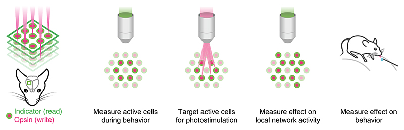
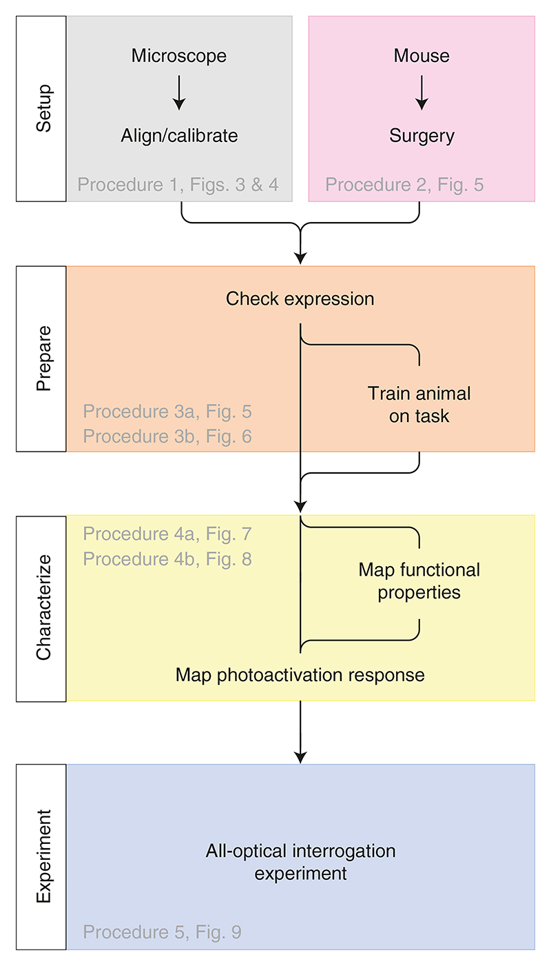
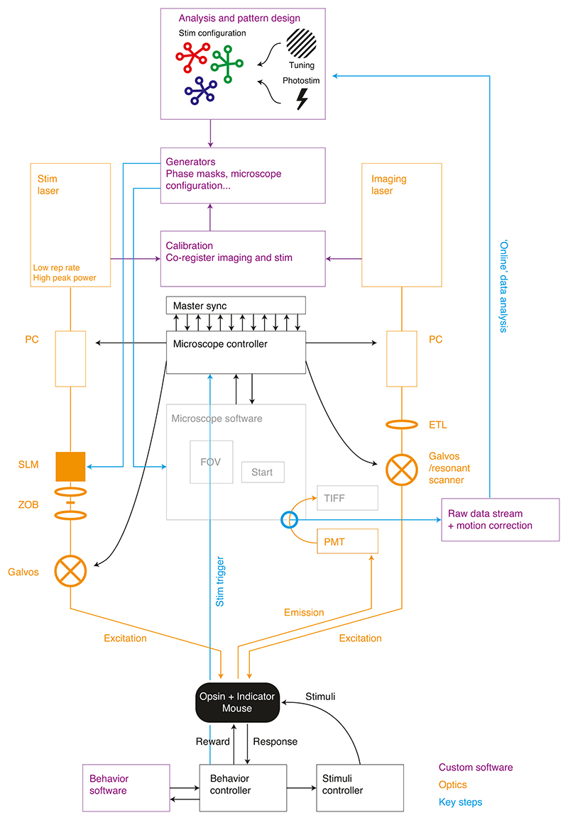
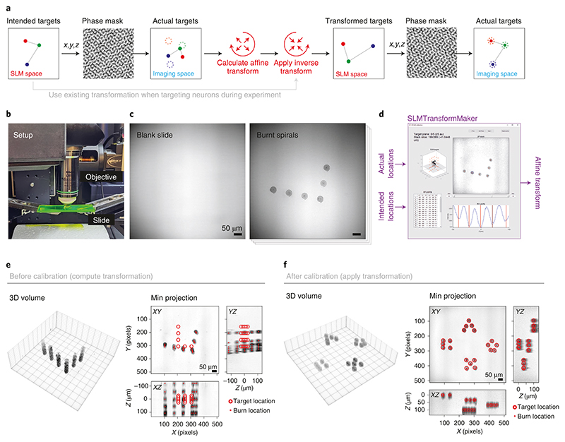
Recent advances combining two-photon calcium imaging and two-photon optogenetics with computer-generated holography now allow us to read and write the activity of large populations of neurons in vivo at cellular resolution and with high temporal resolution. Such 'all-optical' techniques enable experimenters to probe the effects of functionally defined neurons on neural circuit function and behavioral output with new levels of precision. This greatly increases flexibility, resolution, targeting specificity and throughput compared with alternative approaches based on electrophysiology and/or one-photon optogenetics and can interrogate larger and more densely labeled populations of neurons than current voltage imaging-based implementations. This protocol describes the experimental workflow for all-optical interrogation experiments in awake, behaving head-fixed mice. We describe modular procedures for the setup and calibration of an all-optical system (~3 h), the preparation of an indicator and opsin-expressing and task-performing animal (~3-6 weeks), the characterization of functional and photostimulation responses (~2 h per field of view) and the design and implementation of an all-optical experiment (achievable within the timescale of a normal behavioral experiment; ~3-5 h per field of view). We discuss optimizations for efficiently selecting and targeting neuronal ensembles for photostimulation sequences, as well as generating photostimulation response maps from the imaging data that can be used to examine the impact of photostimulation on the local circuit. We demonstrate the utility of this strategy in three brain areas by using different experimental setups. This approach can in principle be adapted to any brain area to probe functional connectivity in neural circuits and investigate the relationship between neural circuit activity and behavior.

Fig. 1. Conceptual goals of all-optical interrogation experiments.

Schematic diagram illustrating the basic elements of all-optical interrogation studies, showing the typical sequence used in an experiment. Indicators are used to read neural activity (both to identify cells active during a behavior/sensory manipulation and to measure any influence of all-optical interrogation on the local network; second and fourth images from the left), and opsins are used to write neural activity (middle image).

Fig. 2. Overview of experimental steps.

Essential steps, common to all all-optical experiments. The microscope must be aligned and calibrated before use. Animals used for experiments are engineered to express an activity indicator and opsin in specific neuronal populations. The expression of these constructs is assessed. Animals are (optionally) trained on a behavioral task. Neural responses to a stimulus/task variable of interest are mapped. Neural responses to photostimulation are mapped to identify photostimulatable cells. Finally, an experiment can be performed whereby functionally characterized neurons are targeted for photostimulation during a behavior of interest.

Fig. 3. System diagram.

To perform all-optical experiments, custom software is used to generate stimulation patterns targeted to neurons of interest as identified by analysis of imaging data. The stimulation patterns are generated in the form of files to load into different microscope software modules interfacing with the optical components and require the use of predetermined calibrations. The stimulation pattern files configure the system such that external triggers (e.g., from a behavioral experiment) can trigger the stimulation of particular neurons by determining the diffraction pattern caused by the SLM and driving power-modulation devices as well as galvanometer mirrors. ETL, electrically tunable lens; Galvos, galvanometers; PC, computer; PMT, photomultiplier tube; Photostim, photostimulation; rep, repetition; SLM, spatial light modulator; Stim, stimulation; sync, synchronization; ZOB, zero-order block.

Fig. 4. SLM calibration: mapping photostimulation targets to imaging coordinates.

a, Without calibrating the SLM coordinates, the intended coordinates converted into the diffraction pattern generated by the SLM (via its displayed phase mask) will focus at arbitrary locations of the imaging FOV, precluding accurate targeting of precise neurons. By mapping the transformation between programmed SLM coordinates and ultimate location on the imaging FOV (usually by a collinearity-preserving affine transformation), the inverse can be applied, allowing for precise targeting of neurons. b, Photograph of a fluorescent plastic slide, used for calibration, imaged by the microscope objective. c, Images of the fluorescent slide acquired by the imaging pathway (left) and the same slide after programming the SLM and burning the resulting spots into the slide by spiral scanning (right). d, Software (SLMTransformMaker) is used to compute the transformation between SLM target coordinates and the imaging FOV locations of those SLM spots after burning them into a plastic slide. e, 3D projection of a volumetric stack taken of the burnt SLM spots (burnt on five axial planes) acquired for the calibration process. f, 3D projection of a different set of SLM patterns, but after calibration, demonstrating successful targeting to intended locations. Min projection = minimum intensity projection.

Fig. 5. Inducing and checking expression of all-optical constructs.

a, Strategies for achieving co-expression of all-optical constructs. b, Co-expression of all-optical constructs in superficial primary somatosensory and visual cortices (L2/3 S1 and V1). Left, experimental prep schematic; a chronic imaging window is installed on the cortical surface with either dual adeno-associated virus (AAV) expression of GCaMP and C1V1 (S1) or AAV expression of C1V1 in GCaMP transgenic mice (V1). Two right-hand images, example of healthy co-expression. c, Co-expression of all-optical constructs in deep cortex (L5 V1). Left, experimental preparation schematic; a chronic imaging window is installed on the cortical surface of L5-Cre transgenic mice injected with FLEX-C1V1 and FLEX-GCaMP. Right, example of healthy co-expression. d, Co-expression of all-optical constructs in subcortical structures (hippocampal CA1 and CA3). Left, experimental preparation schematic; cortical aspiration combined with a canula + chronic imaging window in CA1/CA3-Cre transgenic mice injected with FLEX-C1V1 and FLEX-GCaMP. Two right-hand images, example of healthy co-expression. AP, antero-posterior; bregma, junction point of the coronal and sagittal sutures of the skull; DV, dorso-ventral; lambda, junction point of the lambdoid and sagittal sutures of the skull; ML, medio-lateral.

Fig. 6. Choosing an appropriate behavioral paradigm.

a, Example of a visual detection behavior. Top, task schematic; mice are required to report the presence of a randomly oriented drifting grating on a monitor by licking for a sucrose reward at an electronic lickometer. Bottom, sorted lick raster vertically stacking poststimulus epochs indicating the stimulus duration (black horizontal bar along x-axis), first lick on each trial (black dot) and subsequent trial licks (gray dots). Task performance is indicated by the color bar on the right, where color at each vertical position indicates performance on the corresponding trial in the trial raster to the left. Green, correct response (lick on grating trials; withhold on catch trials); red, incorrect response (lick on catch trials); gray, miss (no lick on grating trials). Note that because this animal is well trained, all trials are correct (green). Note also that trials were delivered pseudorandomly but sorted for display. N = 1 mouse, 1 training session, 367 trials. b, Example of a delay whisker discrimination behavior. Top, task schematic; mice are required to report which whisker pad receives the highest amplitude sinusoidal piezo vibration of two simultaneously delivered bilateral whisker stimuli by licking for sucrose rewards at one of two lickometer ports after an auditory tone Go cue signaling the end of a 1.5-s delay period after stimulus onset. Bottom, sorted lick raster vertically stacking poststimulus epochs; the conventions are the same as in a except that right and left licks are colored red and blue, respectively. As in a, task performance is indicated by the color bar on the right with slightly different color conventions. Green, correct response (lick left on left whisker stimulation trials; lick right on right whisker stimulation trials); red, incorrect response (lick right on left whisker stimulation trials; lick left on right whisker stimulation trials); gray, miss (no lick on either trial type). Note that because this animal is well trained, almost all trials are correct for both contingencies (green). Note also that trials were delivered pseudorandomly but sorted for display. N = 1 mouse, 1 training session, 101 trials. c, Example of a complex spatial navigation paradigm. Top, task schematic; mice are head-fixed on a cylindrical treadmill that controls movement through a virtual linear world displayed on three surrounding monitors. They spawn at the start of the virtual track and are required to run the length of the track before stopping and licking in the designated reward zone. Middle, virtual linear track indicating task features, start zone and reward zone. Note that the track running continuously left to right is a top-down view, whereas landmarks/objects rising from this are side view. Bottom, position along track, speed, lick times and reward deliveries for successive laps along the track. N = 1 mouse, 1 training session, 6 laps along track. Go cue, go cue tone epoch; Catch, catch trials (no stimulus/cue delivered); Grating, stimulus trials on which a visual grating was displayed; Left whiskers, trials on which left whiskers were stimulated; Resp win, behavioral response (lick) window epoch; Right whiskers, trials on which right whiskers were stimulated; Stim, stimulus epoch; Stim L, left whisker stimulus epoch and amplitude; Stim R, right whisker stimulus epoch and amplitude.

Fig. 7. Mapping functional responses online.

a, Example workflow for collection and fast online analysis of functional responses. Key optimizations that allow same-session analysis are (i) online motion correction in real time, which eliminates lengthy post-acquisition motion-correction times, and (ii) generation of stimulus-triggered average (STA) images, which intuitively map response strengths and tunings onto the spatial locations of cells. b, STA image generated from widefield calcium imaging data acquired in primary visual cortex (V1) as a contrast-reversing checkerboard (10°) drifted horizontally across a gray screen (25°/s) positioned in front of the contralateral eye. Pixels are colored by the azimuth that elicited the strongest response. The two-photon imaging volumetric FOV used for c and d is indicated. c, STA images generated from one plane in the two-photon imaging volumetric FOV indicated in a (L2/3 V1) as Gabor patches (30°) of drifting sinusoidal gratings (0.04 cycles/°) of four orientations (0°, 45°, 90° and 135°) were presented to the contralateral eye. Pixels are colored by the orientation that elicited the strongest response. d, Left, extracted traces showing single trial responses to stimuli indicated by vertical colored lines (color conventions are the same as in c; dashed lines are stimuli in the opposite direction to the solid lines). Right, average poststimulus response amplitude. Note that in both heatmaps, neurons have been sorted by preferred stimuli. e, Indicator expression image in primary somatosensory cortex (S1) (grayscale) overlaid with a thresholded STA image heatmap (cyan) acquired during vibration of the C2 whisker. The two-photon imaging volumetric FOV used for f and g is indicated. f, STA image generated from one plane in the two-photon imaging volumetric FOV indicated in e (L2/3 S1) as each of four whiskers were stimulated individually (C1, C2, D2 and D1). Note that this is a composite image combining data from four separate movies, one for each whisker. g, Left, extracted traces showing single trial responses to stimuli indicated by vertical colored lines (color conventions are the same as in f). Right, average poststimulus response amplitude. Note that in both heatmaps, neurons have been sorted by preferred stimuli. h, STA image generated from one plane in the two-photon imaging volumetric FOV in hippocampal CA1 (animal genotype: Emx-Cre × CaMKII-tTa × GCaMP6s). Data were acquired as animals ran along a virtual linear track. Color indicates the position along the virtual track that elicited the strongest response, and color intensity indicates the response magnitude. i, Same as h but in a hippocampal CA3 FOV (animal genotype: Grik4-Cre × CaMKII-tTa × GCamP6s). j, Left, extracted traces from neurons in i showing single trial responses (bottom heatmaps) as an animal ran laps along the virtual linear track (top trajectories). Right, response of all neurons averaged across laps. Note that in both heatmaps, neurons have been first divided into those that are spatially modulated (bottom) and those that are not (top) and sorted within those pools by preferred firing location (place field). Avg., average; ROI, region of interest.

Fig. 8. Mapping photoactivatable neurons.

Panels a and b provide an overview, panels c and d show the workflow, panels e–h show a worked example and further examples are provided in panel i. a, To stimulate one group of cells, the galvanometer mirrors first move to the centroid of the target neurons. The SLM displays a phase mask resulting in diffraction of the beam focusing onto the cells of interest. To stimulate the cells, the power-modulation device permits light transmission and controls the intensity, and the galvanometer mirrors simultaneously move all the diffracted spots in a spiral over the cell bodies of interest. After stimulation, the response can be analyzed. b, To stimulate all cells in the FOV, sequential stimulation of smaller groups is required. c, The workflow. First, an FOV is loaded and analyzed, and ROIs are found/selected and then clustered into groups that will be stimulated one after the other. To drive the microscope system to perform the stimulation as described in a, various files are required to configure the subsystems, including the positioning of the galvanometer mirrors, the SLM phase masks and a trial sequence listing the stimulation order. d, A voltage command is sent from external hardware to trigger the delivery of a photostimulation. The trigger will update the SLM phase mask, move the galvanometer into position, turn on the power modulation and start the galvanometer spiral. e, Software used to design photostimulation mapping experiments. The workflow is as follows: loading FOV images, selecting ROIs, designing the grouping, configuring the stimulation parameters and finally exporting the files to load into microscope control systems. f, Protocol to run the photostimulation mapping experiment: load the generated microscope configuration files, record a time-series movie (optionally performing online motion correction) and trigger the stimulations throughout the recording. After acquisition, the data are analyzed to identify responsive cells. g, Example STA images of the response after photostimulation of three groups (stimulated 1 s after each other). The right panel shows a composite image in which the hue corresponds to pattern number and the intensity corresponds to the response magnitude. h, Activity traces extracted from ROIs targeted in the same experiment as in g; stimulations are indicated by vertical colored lines extending through the neurons that were targeted in a particular pattern. The right panel shows STA traces. i, Example STA images for the response to photostimulation mapping experiments as in g in various brain regions (labeled on each image). Colors represent groups of neurons photostimulated concurrently. config, configuration; Galvo, galvanometer.

Fig. 9. A worked example: probing the perceptual salience of sensory-responsive neurons in the L2/3 barrel cortex by using targeted two-photon optogenetic stimulation.

a, Schematic illustrating the general workflow from acquisition of characterization data to generation of components necessary to perform an all-optical experiment. b, Sequence of steps necessary to acquire relevant characterization data in this worked example. Left, C2 whisker stimulation during widefield calcium imaging of S1 allows identification of the C2 whisker barrel used as the two-photon FOV going forward. Two-photon expression images of opsin (middle left, top), indicator (middle left, middle) and two-photon imaging movies acquired during whisker stimulation (middle left, bottom) are used for selection of opsin-expressing ROIs (middle right, top) as a reference image for real-time motion correction (middle right, middle) and to generate functional GCaMP-expressing ROIs via online Suite2p (middle right, bottom) with opsin and Suite2p centroids and then used to generate two-photon photostimulation targets (middle). Only targets in the central region of the FOV are included (dashed white border), and these are divided into four groups of 50 neurons (colors). These groups are then used for the Naparm protocol, which is subsequently concatenated with previously acquired sensory characterization movies and run through online Suite2p. Right, This yields extracted traces from Suite2p ROIs that can be used to generate sensory and photostimulus STAs. c, Thresholds (gray dashed lines) are set on the sensory and photostimulus responses to find photostimulable neurons that also respond to sensory stimuli. d, Overlay of sensory and photostimulus response types onto the Suite2p ROI image, highlighting the location of target neurons (dashed circles). e, Target coordinates for two photostimulus trial types, one stimulating 100 random neurons (trial type 1) and another stimulating just the 6 sensory-responsive neurons (trial type 2; see c and d), are embedded into a behavioral task paradigm via a custom GUI that allows the binding of specific phase masks with trial types and the organization of trial types into a sequence of trials for a given behavioral session. Note that panels are for schematic purposes; details will vary per experiment. f, Top, task schematic; mice are required to report the detection of two-photon photostimulation targeted to ensembles of neurons (500-ms duration; 10 × 20-ms spirals at 20 Hz) by licking at an electronic lickometer for sucrose rewards in a 1-s response window after the onset of photostimulation, or to withhold licking on catch trials during which no neurons were photostimulated. Bottom, sorted lick raster split by trial type from the behavioral session immediately after the characterization in b–e. Trials were delivered pseudorandomly but are sorted for display. Stimulus durations are shown as colored bars at the bottom of the raster. g, Proportion of trials on which the animal licked, and therefore putatively detected photostimulation, for each trial type. Error bars are binomial. N = 1 session; 58 random trials, 29 sensory trials, 78 catch trials. h, Reaction time for each trial type. Error bars are s.d.. N = 1 session; 58 random trials, 29 sensory trials, 78 catch trials.

Fig. 10. Two-photon excitation and calibration of safe and effective stimulation parameters.

Panels a–c show laser terminology, panels d and e show photostimulation efficiency and panels f–j show photostimulation safety. a, Two-photon excitation compared to one-photon excitation. b, Diagram illustrating key parameters of pulsed lasers used for both imaging and photostimulation applications. c, Hypothetical comparison between two lasers with the same average power and pulse width, but with a different repetition rate (and thus peak power). d, FOV fluorescence image before and after photostimulation of a 30-cell ensemble. Animals were wild types virally expressing AAV1-hSyn-GCaMP6s and AAVdj-CaMKII-C1V1. Scale bar represents 100 μm. e, Stimulation of 10-cell groups (prefilter for responsive neurons) with range of average powers at two different laser repetition rates (indicated in red and black). These groups were stimulated in blocks of increasing powers at one of the two repetition rates. Spiral parameters were as follows: 15-μm diameter and 20-ms duration repeated 5 times at 20 Hz. 10 trials of each stimulation were conducted, with 10 s between each stimulation. Plots show the average response size (ΔF/F) of the targeted ROIs as a function of the average power per cell (measured on the sample), the peak power or the integrated probability of two-photon excitation. Numbers indicate the average power (mW). On the basis of these assessments, 6 mW (3 mW/µm²) per cell (at 2 MHz) was chosen as an effective power to use for our stimulation experiments, given its ability to evoke reliable transients while being safe to not cause noticeable damage (see f–i below). f, To assess phototoxicity, we stimulated single cells with increasing average powers (from 6 to 36 mW at 2-MHz repetition rate). Cells were selected from GCaMP expression images with no knowledge of opsin expression. Various expression strategies were used. tetO refers to transgenic animals expressing GCaMP6s under the tetO system. Spiral parameters were as follows: 15-μm diameter and 20-ms duration repeated 5 times at 20 Hz. 10 trials of each stimulation were conducted, with 10 s between each stimulation. Images show the FOV of GCaMP expression before and after the single-cell stimulation protocol. Note the bright filled appearance of the targeted cells after the protocol, indicating that damage occurred by the higher stimulation powers. Scale bar represents 100 μm. g, Outline of the calibration protocol. We select one parameter at a time, keeping all others constant. We perform 10 trials at a given value of that parameter and then increment it and acquire 10 more trials, repeating until we reach the maximum value to be tested. Subsequent analysis is used to select the power that was effective (resulted in activation of neurons) and also safe (no changes in baseline fluorescence). If there are multiple parameters to be tested, we would then proceed in a similar fashion with the next parameter. h, Average response size of the targeted cells across trials and blocks of increasing power. Responses all tend to decrease within a block, probably because of opsin desensitization. The large ‘responses’ at 30 and 36 mW (22 and 26 mW/µm²) are a result of photoablation. i, Average baseline fluorescence of the targeted cells across trials and blocks of increasing stimulation power. We used the baseline fluorescence as an indicator of cell health, with increases (that were not the tail end of GCaMP transients) representing an undesirable change. Note the strong increase after a few trials at 18 mW (10 mW/µm²), indicating that damage is accumulating in the targeted cells with this stimulation power. In this panel, it should also be noted that we find that opsin expression lowers the power threshold required to cause increases in baseline brightness (c.f. green TetO + None data with all other conditions). To our knowledge this has not been reported before, but it is possible that this results from the impact on cell health caused by the increased metabolic load imposed by additional opsin expression. j, An example of intentional photoablation of a multiple-cell ensemble, by using a very-low-repetition-rate (0.2 MHz) laser. 2PE prob., two-photon excitation probability.

References

1. Jacobs AL, et al. Ruling out and ruling in neural codes. Proc Natl Acad Sci USA. 2009;106:5936–5941. - PMC - PubMed
1. Panzeri S, Harvey CD, Piasini E, Latham PE, Fellin T. Cracking the neural code for sensory perception by combining statistics, intervention and behavior. Neuron. 2017;93:491–507. - PMC - PubMed
1. London M, Roth A, Beeren L, Häusser M, Latham PE. Sensitivity to perturbations in vivo implies high noise and suggests rate coding in cortex. Nature. 2010;466:123–127. - PMC - PubMed
1. Histed MH, Maunsell JHR. Cortical neural populations can guide behavior by integrating inputs linearly, independent of synchrony. Proc Natl Acad Sci USA. 2014;111:E178–E187. - PMC - PubMed
1. Gollisch T, Meister M. Rapid neural coding in the retina with relative spike latencies. Science. 2008;319:1108–1112. - PubMed
Publication types