Traveling waves of an FKPP-type model for self-organized growth

Abstract

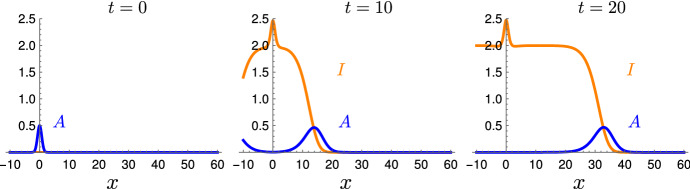
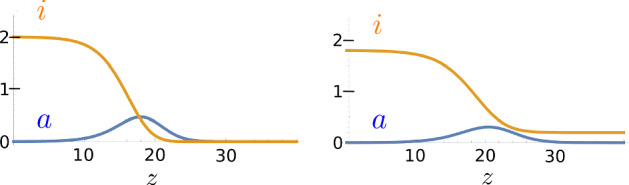
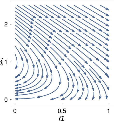
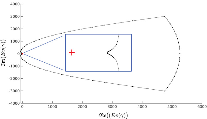
We consider a reaction-diffusion system of densities of two types of particles, introduced by Hannezo et al. (Cell 171(1):242-255.e27, 2017). It is a simple model for a growth process: active, branching particles form the growing boundary layer of an otherwise static tissue, represented by inactive particles. The active particles diffuse, branch and become irreversibly inactive upon collision with a particle of arbitrary type. In absence of active particles, this system is in a steady state, without any a priori restriction on the amount of remaining inactive particles. Thus, while related to the well-studied FKPP-equation, this system features a game-changing continuum of steady state solutions, where each corresponds to a possible outcome of the growth process. However, simulations indicate that this system self-organizes: traveling fronts with fixed shape arise under a wide range of initial data. In the present work, we describe all positive and bounded traveling wave solutions, and obtain necessary and sufficient conditions for their existence. We find a surprisingly simple symmetry in the pairs of steady states which are joined via heteroclinic wave orbits. Our approach is constructive: we first prove the existence of almost constant solutions and then extend our results via a continuity argument along the continuum of limiting points.

Keywords: Cellular organization; Continum of fixed points; Developmental biology; Pattern formation; Reaction–diffusion equation; Traveling wave.

Fig. 1

Simulation of the Reaction–Diffusion System (1.1) for $r=0$. Given a small initial heap of active particles $A(x,0)=1/2exp(-x^2)$ and $I(x,0)=0$, two identical traveling fronts arise, the right one is shown. After the separation of the two fronts away from the origin, the density of the remaining inactive particles is given by $I=2$ and the front moves asymptotically with speed $c=2$

Fig. 2

Two different traveling waves with speed $c=2$. The limits of the left wave are given by $i_{-\infty }=2$ and $i_{+\infty }=0$. The limits of the right wave are given by $i_{-\infty }=1.8$ and $i_{+\infty }=0.2$

Fig. 3

Two-dimensional phase portrait of (a, i) of traveling waves (2.1) for $c=2$ and $r=0$, omitting the coordinate $b=a^{\prime }$. A unique trajectory emerges from each point in $S_{-\infty }$ (where $i_{-\infty }>1$) in positive direction of a and converges to $S_{+\infty }$ (where $i_{+\infty }<1$). Notice the correspondence $i_{-\infty }+i_{+\infty }=2$ of the limits

Fig. 4

Phase portrait of (a, b) of the Wave Eq. (2.1) if we impose a fixed value of $i(z)=0$, see also Sect. 5. The choices of c change the type of convergence towards the origin: spiraling for $c=1$, one stable manifold with eigenvalue $-c/2$, which has algebraic multiplicity 2 and geometric multiplicity 1 for $c=2$, two stable manifolds for $c=3$

Fig. 5

The phase plot of $(\overline{a},\overline{b})$ following Eq. (5.1), displayed for several values of i and c. The only two fixed points are (0, 0) and $(1-i,0)$. For $i\ge i_c$, the orange triangles $T_c(i)$ are invariant regions of Dynamics (5.1), see Prop. 5.3. They increase in $-i$: the point $(1-i,0)$ moves to the right and the two internal angles ${\gamma }_l(i)$ and ${\gamma }_r(i)$ increase. In the third case, $i<i_c$ implies that the system spirals around (0, 0) while converging

Fig. 6

Trajectories of $a(z),i(z)$ of the Wave System (2.1) for $c=2,r=0$. Initial values are $b(0)=0,i_0=0.5$, and $a_0$ such that $a_0\in [0,a^{\ast }(i_0)\approx 0.42]$. The upper bound $a^{\ast }$ is given in Definition 6.8. Trajectories with such initial data converge and stay non-negative, since $i(z)\ge i_c$

Fig. 7

Numerical evaluation of the Evans-function (B6) $Ev(\gamma )$ for $r=0$ and $\gamma$ on the boundary of the Domain S, defined in (B7). The Evans-function for $r=1$ is very similar. The origin is marked with a small red cross. The graph does not enclose the origin and it can visually be seen that its winding number is equal to zero. We conclude that the Region S contains no zeros of $Ev(\gamma )$

References

-
- Arumugam G, Tyagi J. Keller–Segel chemotaxis models: a review. Acta Appl Math. 2020;171(1):6. doi: 10.1007/s10440-020-00374-2. - DOI
- Barker B, Humpherys J, Zumbrun K (2015) STABLAB: A MATLAB-Based Numerical Library for Evans Function Computation. Available in the github repository under nonlinear-waves/stablab
- Berestycki H, Nicolaenko B, Scheurer B. Traveling wave solutions to combustion models and their singular limits. SIAM J Math Anal. 1985;16(6):1207–1242. doi: 10.1137/0516088. - DOI
- Berestycki J, Brunet E, Derrida B. A new approach to computing the asymptotics of the position of fisher-kpp fronts. Europhys Lett (EPL) 2018;122(1):10001. doi: 10.1209/0295-5075/122/10001. - DOI
Publication types
MeSH terms
LinkOut - more resources
Full Text Sources