Time-Frequency Representations of Brain Oscillations: Which One Is Better?

Abstract

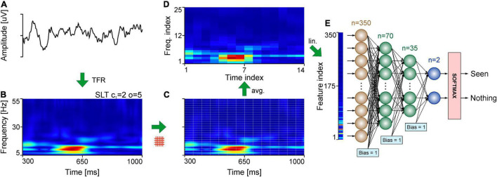
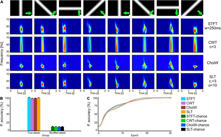
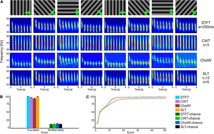
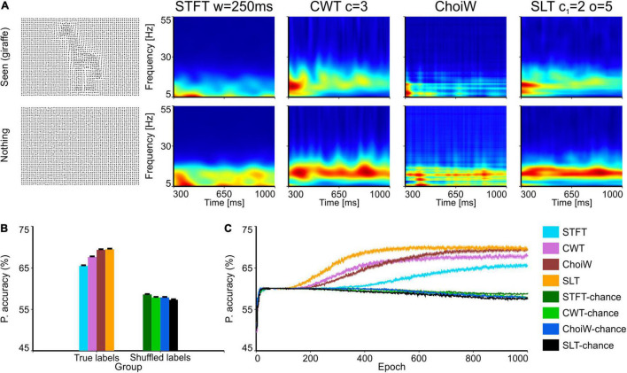
Brain oscillations are thought to subserve important functions by organizing the dynamical landscape of neural circuits. The expression of such oscillations in neural signals is usually evaluated using time-frequency representations (TFR), which resolve oscillatory processes in both time and frequency. While a vast number of methods exist to compute TFRs, there is often no objective criterion to decide which one is better. In feature-rich data, such as that recorded from the brain, sources of noise and unrelated processes abound and contaminate results. The impact of these distractor sources is especially problematic, such that TFRs that are more robust to contaminants are expected to provide more useful representations. In addition, the minutiae of the techniques themselves impart better or worse time and frequency resolutions, which also influence the usefulness of the TFRs. Here, we introduce a methodology to evaluate the "quality" of TFRs of neural signals by quantifying how much information they retain about the experimental condition during visual stimulation and recognition tasks, in mice and humans, respectively. We used machine learning to discriminate between various experimental conditions based on TFRs computed with different methods. We found that various methods provide more or less informative TFRs depending on the characteristics of the data. In general, however, more advanced techniques, such as the superlet transform, seem to provide better results for complex time-frequency landscapes, such as those extracted from electroencephalography signals. Finally, we introduce a method based on feature perturbation that is able to quantify how much time-frequency components contribute to the correct discrimination among experimental conditions. The methodology introduced in the present study may be extended to other analyses of neural data, enabling the discovery of data features that are modulated by the experimental manipulation.

Keywords: electroencephalography; explainable AI; machine learning; neural oscillations; neurophysiology; time-frequency representation.

FIGURE 1

Analysis pipeline for evaluating TFRs. (A) Example of single trial EEG signal. (B) TFR using the SLT of the EEG signal in panel (A). (C) Slicing of the TFR into time-frequency tiles. (D) Standardization of the TFR tiles using bicubic interpolation. (E) Linearization of the tiled, interpolated TFR in panel (D), fed to the MLP. The example indicates the application of the pipeline for a single trial of the EEG dataset.

FIGURE 2

Intracranial electrophysiology with RF visual stimulation protocol. (A) Table of TFRs where each column corresponds to a particular grating direction (condition) and each row corresponds to one of the time-frequency analysis methods. (B) Average accuracy as measured on the validation set (100 network initializations and dataset splits), with original (true) and shuffled labels (for chance level estimation). (C) Learning curves on the validation set for the original labels group (chance level curves were omitted here but reside at ∼12.5%). Error bars are s.e.m.

FIGURE 3

Intracranial electrophysiology with SRCS visual stimulation protocol (SRCS-1). (A) Table of TFRs where each column corresponds to a particular grating direction (condition) and each row corresponds to one of the time-frequency analysis methods. (B) Average accuracy as measured on the validation set (100 network initializations and dataset splits), with original (true) and shuffled labels (for chance level estimation). (C) Learning curves on the validation set for the original labels group (chance level curves were omitted here but reside at ∼12.5%). Error bars are s.e.m.

FIGURE 4

Intracranial electrophysiology with SRCS visual stimulation protocol (SRCS-2). (A) Table of TFRs where each column corresponds to a particular grating direction (condition) and each row corresponds to one of the time-frequency analysis methods. (B) Average accuracy as measured on the validation set (100 network initializations and dataset splits), with original (true) and shuffled labels (for chance level estimation). (C) Learning curves on the validation set for the original labels group (chance level curves were omitted here but reside at ∼12.5%). Error bars are s.e.m.

FIGURE 5

Electroencephalography data with the Dots 30 stimulation protocol. (A) Table of TFRs where each row corresponds to the participant’s response (“nothing” or “seen”) and each column corresponds to one of the time-frequency analysis methods. First column on the left shows an example of the visual stimulus for a seen shape (a giraffe, top) and nothing (bottom). (B) Average accuracy as measured on the validation set (100 network initializations and dataset splits), with original and shuffled labels for chance level estimation. (C) Average learning curves on the validation set. Error bars are s.e.m.

FIGURE 6

Importance of time-frequency components for distinguishing experimental conditions in the EEG data. (A) Pairwise feature correlation for each method. (B) Top row: increase in MSE (ΔMSE) when features (time-frequency components) are randomly permuted between trials. Bottom row: magnitude of decrease of prediction accuracy (-ΔPAcc) as a result of feature permutation. Larger positive values represent more important features for correct classification.

References

-
- Barredo Arrieta A., Díaz-Rodríguez N., Del Ser J., Bennetot A., Tabik S., Barbado A., et al. (2020). Explainable Artificial intelligence (XAI): concepts, taxonomies, opportunities and challenges toward responsible AI. Inf. Fusion 58 82–115. 10.1016/j.inffus.2019.12.012 - DOI
- Bârzan H., Moca V. V., Ichim A.-M., Muresan R. C. (2021). “Fractional Superlets,” in Proceedings of the 2020 28th European Signal Processing Conference (EUSIPCO). Presented at the 2020 28th European Signal Processing Conference (EUSIPCO), (Amsterdam: EUSIPCO; ). 2220–2224. 10.23919/Eusipco47968.2020.9287873 - DOI
LinkOut - more resources
Full Text Sources