Unsupervised learning for robust working memory

Abstract

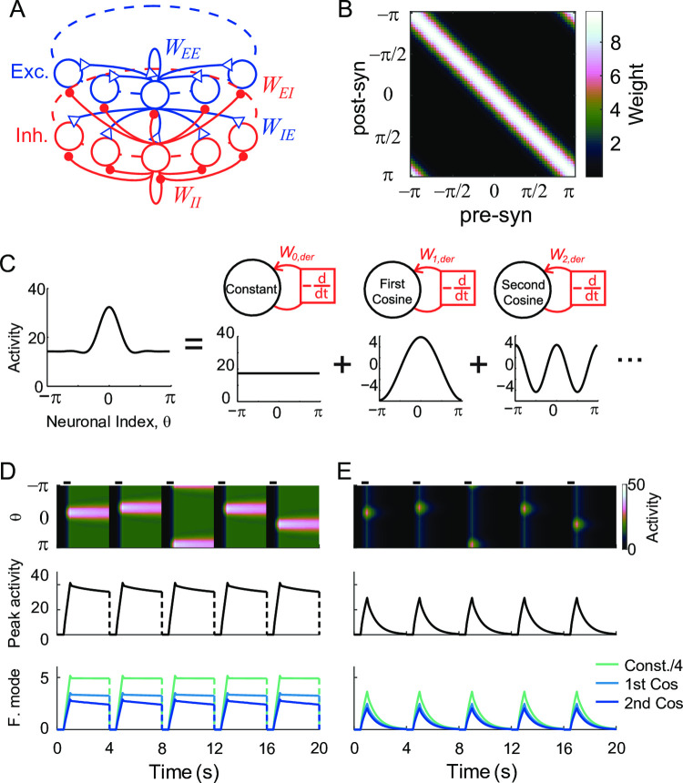
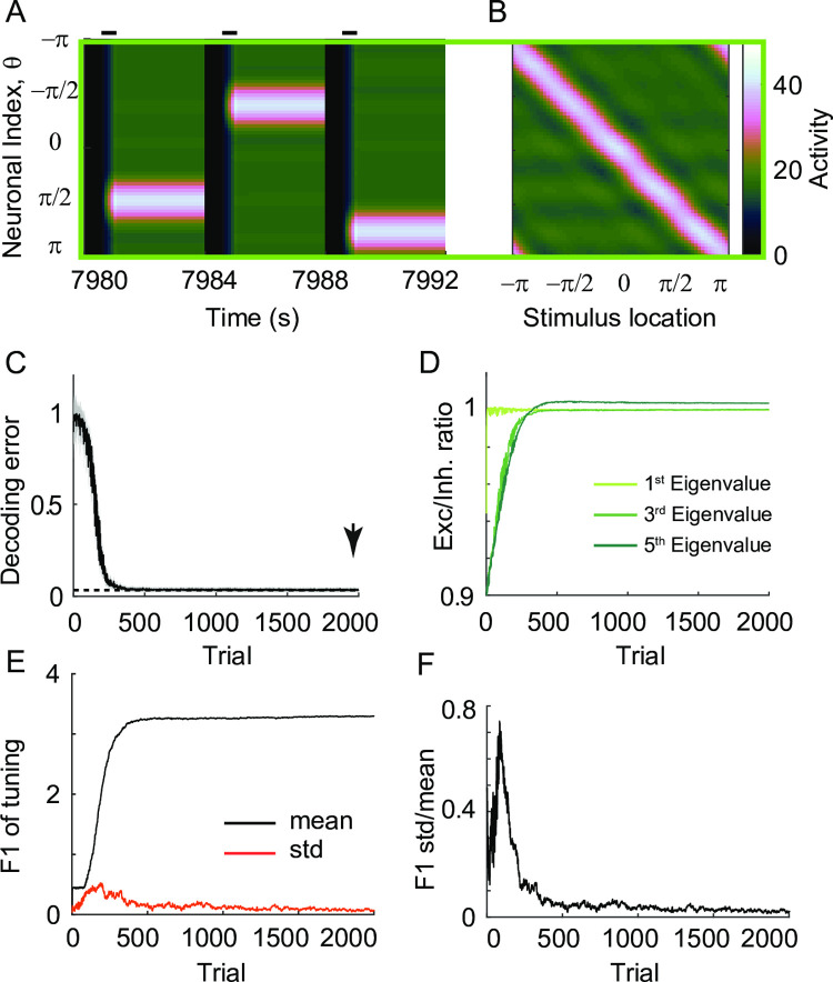
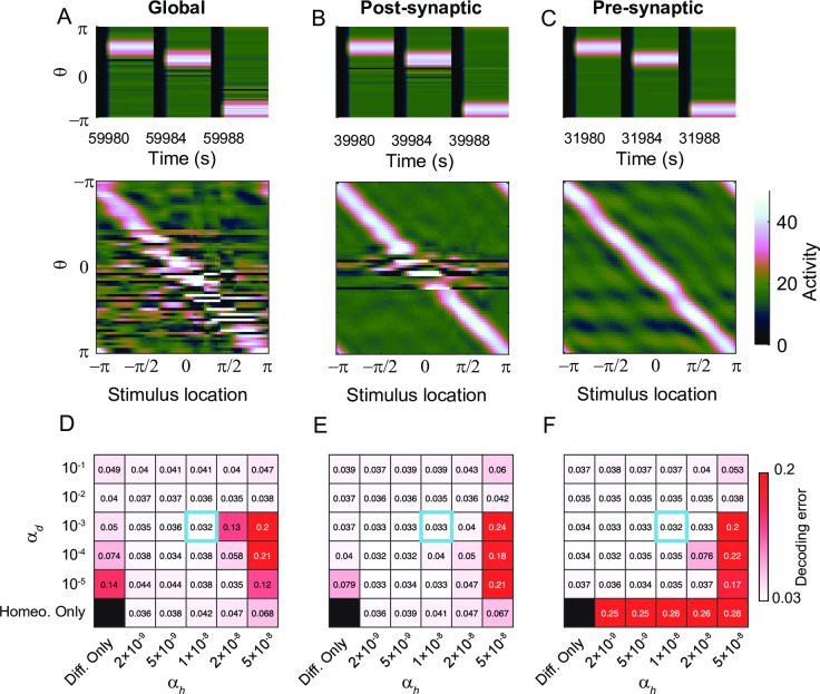
Working memory is a core component of critical cognitive functions such as planning and decision-making. Persistent activity that lasts long after the stimulus offset has been considered a neural substrate for working memory. Attractor dynamics based on network interactions can successfully reproduce such persistent activity. However, it requires a fine-tuning of network connectivity, in particular, to form continuous attractors which were suggested for encoding continuous signals in working memory. Here, we investigate whether a specific form of synaptic plasticity rules can mitigate such tuning problems in two representative working memory models, namely, rate-coded and location-coded persistent activity. We consider two prominent types of plasticity rules, differential plasticity correcting the rapid activity changes and homeostatic plasticity regularizing the long-term average of activity, both of which have been proposed to fine-tune the weights in an unsupervised manner. Consistent with the findings of previous works, differential plasticity alone was enough to recover a graded-level persistent activity after perturbations in the connectivity. For the location-coded memory, differential plasticity could also recover persistent activity. However, its pattern can be irregular for different stimulus locations under slow learning speed or large perturbation in the connectivity. On the other hand, homeostatic plasticity shows a robust recovery of smooth spatial patterns under particular types of synaptic perturbations, such as perturbations in incoming synapses onto the entire or local populations. However, homeostatic plasticity was not effective against perturbations in outgoing synapses from local populations. Instead, combining it with differential plasticity recovers location-coded persistent activity for a broader range of perturbations, suggesting compensation between two plasticity rules.

Fig 1. Recovery of rate-coded persistent activity through differential plasticity.

A: Maintenance of persistent activity through negative-derivative feedback. With balanced excitation and inhibition as well as slower excitation, the network can maintain persistent activity at different rates. The top panel illustrates the schematic of a pulse-like stimulus. The dotted and dash-dotted curves in both top and bottom panels represent stimulus and activity with double and half the input strengths compared to the solid one. B: Schematics of differential plasticity in the excitatory feedback. C-D: Recovery of persistent activity (C) and E-I balance under differential plasticity (D) after perturbations in connectivity strengths. E-F: Activities with 10% perturbation (E) and after the recovery (F). The time axis is in the unit of intrinsic time constant τ, and one trial is composed of the stimulus presentation, delay period, and an inter-trial interval. Shaded areas represent the delay period during which the plasticity occurs.

Fig 2. Recovery dynamics dependence on learning parameters under differential plasticity.

A: Phase-plane of activity r and synaptic strength of recurrent excitation W_exc. The small black arrows represent a vector field for the dynamics of r and W_exc, described in Eq 2. The red curve is a trajectory starting from 10% perturbation in W_exc, that is, W_exc = 0.9W_inh with W_inh = 500. During the stimulus presentation, the trajectory jumps horizontally, and input strengths vary randomly across trials. The big arrows indicate the effects of changing the learning speed α or W_inh (blue vertical) and relative mean input strengths c (magenta horizontal). B-E: Dependence of recovery speed on learning and network parameters. The minimum number of trials for W_exc to reach up to 0.99W_inh, that is, about 1% from perfect tuning was obtained by varying α (B), c (C), W_inh (D), perturbation strength p (E). All parameters change from 50% to 200% of those used in Fig 1.

Fig 3. Recovery of rate-coded persistent activity through homeostatic plasticity.

A: Schematics of homeostatic plasticity scaling the strengths of incoming synapses to achieve the target firing rate r₀. B-C: Recovery of E-I balance after perturbations in connectivity strengths (B) and maintenance of persistent activity at the different levels after the recovery (C).

Fig 4. Sensitivity of homeostatic learning rule on learning parameters.

A-B: Dependence of final balance ratio W_exc/W_inh on r₀ (A) and α (B). After reaching the steady state, W_exc/W_inh was averaged over the trials whose mean and standard deviation were shown as red curve and graded area. C-D: Evolution of W_exc/W_inh over trials (top) and the activity after reaching the steady state (bottom) for lower r₀ (C) and higher r₀ (D) compared to that in Fig 3B and 3C. E: Sensitivity to learning speed α. For a faster learning rate, the homeostatic plasticity leads to the oscillation even for properly tuned r₀, leading to a larger standard deviation (square in B) compared to a slower learning rate (circle in B corresponding to Fig 3B and 3C).

Fig 5. Location-coded persistent activity and its disruption under perturbation of tuning.

A: Schematics of the spatial structure of network for location-coded memory. We considered that both excitatory and inhibitory neurons are organized in a columnar structure where each column consists of neurons with a similar preferred feature of the stimulus. Blue and red represent excitatory and inhibitory connections, respectively. B: Example connectivity matrix showing symmetry under translation. We considered the memory neurons encode the spatial information during the delay period, which lies on a circle, represented by θ ranging between -π and π. We assumed that before perturbation, the synaptic strengths depend only on the difference between feature preference of post and presynaptic neurons. C: Decomposition of spatially patterned activity into Fourier modes under translation-invariance. Figure adapted from [13]. D-E: Location-coded persistent activity under E-I balance (D) and its disruption under 10% global perturbation in the E-to-E connection (E). The upper panels show the activity of all neurons during five consecutive trials with each neuron labeled by its preferred feature. The middle panels show the activity of the neuron at the stimulus center and the lower panels show the activity of 3 Fourier modes with the constant mode shrunk by a factor of 1/4 for better visualization.

Fig 6. The effect of differential plasticity under small global perturbation.

A: Recovery of location-coded memory under differential plasticity with learning rate α_d = 10⁻³ and 10% global perturbation in the E-to-E connections. B: Activity pattern at the end of the delay period after the recovery. With the connectivity frozen at trial 2000 (arrow in C), the spatial pattern of activity at the end of the delay period was shown for different stimulus locations. C: Decrease of decoding error with learning. An individual trial refers to one memory task with a specific stimulus location. For each trial, we took the snapshot of activity at the end of the delay period as in B and quantified the mean of the decoding error using the population vector decoder (black curve; Methods) and the standard error of the mean (grey shaded area). Dashed line indicates decoding error before perturbation. D: Recovery of E-I balance for different Fourier modes. The eigenvector decomposition reveals the effective time constant of decay and recovery of E-I balance in different Fourier modes (S2 Fig; Methods). E: Mean (black) and standard deviation (red) of spatial selectivity across neurons quantified by the first Fourier component of each neuron’s tuning curve at the end of the delay period. F: Normalized standard deviation of spatial selectivity in (E), where its decrease with learning indicates recovery of translation-invariance.

Fig 7. The effect of differential plasticity under various levels of global perturbation and learning rates.

A-B: Activity pattern during three successive trials (A) and at the end of delay period for various stimulus locations (B) after reaching the steady state with α_d = 10⁻³ and 30% global perturbation (yellow box in E,F). C-D: Evolution of decoding error (C) and normalized deviation of spatial selectivity (D). E-F: Heatmap showing decoding error (E) and normalized deviation of spatial selectivity (F) after reaching steady state under different learning rates α_d and perturbation strengths p. The green box and yellow box correspond to the case showing recovery of translation-invariance (Fig 6) and the case with breaking-down of translation-invariance (Fig 7A–7D).

Fig 8. The effect of homeostatic plasticity under global perturbation.

A: Recovery of location-coded memory under homeostatic plasticity with target rate r₀ = 20, learning rate α_h = 10⁻⁸ and perturbation strength p = 30% in the E-to-E connections (arrow in D-F). B: Activity pattern at the end of the delay period after the recovery (arrow in C). C: Decrease of decoding error (black) and preservation of translation-invariance (red) with learning. D-F: Dependence of postsynaptic E-I ratio on target firing perturbation strength p (D), rate r₀ (E), and learning rate α_h (F). Note that, unlike Fig 6D, the E-I ratio is not defined by eigenvalue or in the Fourier domain. As homeostatic plasticity modifies all incoming synapses of a neuron with a common factor, we quantified the E-I ratio compared to that before perturbation for each neuron. The mean is shown in black, and the standard deviation across neurons is shown in grey shaded area. G-I: Decoding error and normalized deviation of spatial selectivity for various p (G), r₀, (H), α_h (I).

Fig 9. The effect of differential and homeostatic plasticity under postsynaptic perturbations.

A: Schematics of postsynaptic perturbations where the rows of the connectivity matrix are multiplied by different scaling factors. Perturbation is centered at θ = 0 and bell-shaped. B: Activity pattern under 30% postsynaptic perturbations before any plasticity. C-D: Activity pattern shaped by the differential (C) and homeostatic (D) plasticity. The learning parameters used here are α_d = 10⁻³, α_h = 10⁻⁸, and r₀ = 20. E-F: Decoding errors (black) and normalized deviation of spatial selectivity (red) for different perturbation strengths after applying differential (E) and homeostatic (F) plasticity. Perturbation strength marked by arrow is shown in C-D.

Fig 10. The effect of differential and homeostatic plasticity under presynaptic perturbations.

A: Schematics of presynaptic perturbations where the columns of the connectivity matrix are multiplied by different scaling factors. B-F: Same as in Fig 9B–9F but under 30% presynaptic perturbation (B-D) and the same learning parameters.

Fig 11. The effect of the combination of differential and homeostatic plasticity.

A-C: Recovery of location-coded persistent activity under combined plasticity after 30% global (A), postsynaptic (B), and presynaptic perturbation (C) with the same learning parameters in Figs 9 and 10. The combined plasticity shows better performance compared to the recovery with differential plasticity alone under global perturbation (Fig 7A–7D), under local postsynaptic perturbation (Fig 9C) and the recovery with homeostatic plasticity alone under local presynaptic perturbation (Fig 10D). D-F: Heatmap of the final decoding error under various learning speeds. See S7–S9 Figs for normalized deviation of spatial selectivity and the activity pattern from which decoding errors and spatial selectivity variability were derived.

References

1. Knierim JJ, Zhang K. Attractor dynamics of spatially correlated neural activity in the limbic system. Annu Rev Neurosci. 2012;35: 267–285. doi: 10.1146/annurev-neuro-062111-150351 - DOI - PMC - PubMed
1. Goldman MS, Compte A, Wang XJ. Neural Integrator Models. Encyclopedia of Neuroscience. Elsevier Ltd; 2009. pp. 165–178. doi: 10.1016/B978-008045046-9.01434–0 - DOI
1. Durstewitz D, Seamans JK, Sejnowski TJ. Neurocomputational Models of Working Memory. Nat Neurosci. 2000;3: 1184–1191. doi: 10.1038/81460 - DOI - PubMed
1. Wang XJ. Synaptic reverberation underlying mnemonic persistent activity. Trends Neurosci. 2001;24: 455–463. doi: 10.1016/s0166-2236(00)01868-3 - DOI - PubMed
1. Aksay E, Baker R, Seung HS, Tank DW. Correlated Discharge among Cell Pairs within the Oculomotor Horizontal Velocity-to-Position Integrator. J Neurosci. 2003. doi: 10.1523/JNEUROSCI.23-34-10852.2003 - DOI - PMC - PubMed
Publication types