Multi-omics single-cell data integration and regulatory inference with graph-linked embedding

Abstract

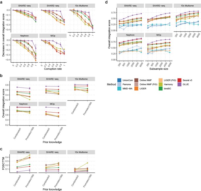
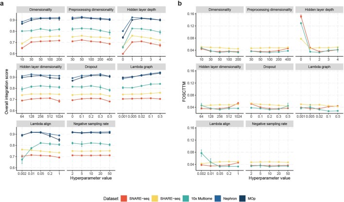
Despite the emergence of experimental methods for simultaneous measurement of multiple omics modalities in single cells, most single-cell datasets include only one modality. A major obstacle in integrating omics data from multiple modalities is that different omics layers typically have distinct feature spaces. Here, we propose a computational framework called GLUE (graph-linked unified embedding), which bridges the gap by modeling regulatory interactions across omics layers explicitly. Systematic benchmarking demonstrated that GLUE is more accurate, robust and scalable than state-of-the-art tools for heterogeneous single-cell multi-omics data. We applied GLUE to various challenging tasks, including triple-omics integration, integrative regulatory inference and multi-omics human cell atlas construction over millions of cells, where GLUE was able to correct previous annotations. GLUE features a modular design that can be flexibly extended and enhanced for new analysis tasks. The full package is available online at https://github.com/gao-lab/GLUE .

Fig. 1. Architecture of the GLUE framework.

Denoting unpaired data from three omics layer as ${\mathbf{X}}_1\in {\mathbb{R}}^{N_1\times ∣{\mathcal{V}}_1∣},{\mathbf{X}}_2\in {\mathbb{R}}^{N_2\times ∣{\mathcal{V}}_2∣},{\mathbf{X}}_3\in {\mathbb{R}}^{N_3\times ∣{\mathcal{V}}_3∣}$, where N₁, N₂, N₃ are cell numbers, and ${\mathcal{V}}_1,{\mathcal{V}}_2,{\mathcal{V}}_3$ are sets of omics features in each layer, GLUE uses omics-specific variational autoencoders to learn low-dimensional cell embeddings U₁, U₂, U₃ from each omics layer. The data dimensionality and generative distribution can differ across layers, but the embedding dimension m is shared. To link the omics-specific data spaces, GLUE makes use of prior knowledge about regulatory interactions in the form of a guidance graph $\mathcal{G}=\left(\mathcal{V},\mathcal{E}\right)$, where vertices $\mathcal{V}={\mathcal{V}}_1\cup {\mathcal{V}}_2\cup {\mathcal{V}}_3$ are omics features. A graph variational autoencoder is used to learn feature embeddings $\mathbf{V}={\left({\mathbf{V}}_1^{\top },{\mathbf{V}}_2^{\top },{\mathbf{V}}_3^{\top }\right)}^{\top }$ from the prior knowledge-based guidance graph, which are then used in data decoders to reconstruct omics data via inner product with cell embeddings, effectively linking the omics-specific data spaces to ensure a consistent embedding orientation. Last, an omics discriminator D is used to align the cell embeddings of different omics layers via adversarial learning. ${\varphi }_1,{\varphi }_2,{\varphi }_3,{\varphi }_{\mathcal{G}}$ represent learnable parameters in data and graph encoders. ${\theta }_1,{\theta }_2,{\theta }_3,{\theta }_{\mathcal{G}}$ represent learnable parameters in data and graph decoders. ψ represents learnable parameters in the omics discriminator.

Fig. 2. Systematic benchmarks of integration performance.

a, Biological conservation score versus omics integration score for different integration methods. b, Overall integration score (defined as 0.6 × biology conservation + 0.4 × omics integration) of different integration methods (n = 8 repeats with different model random seeds). c, Single-cell level alignment error (quantified by FOSCTTM) of different integration methods (n = 8 repeats with different model random seeds). d, Increases in FOSCTTM at different prior knowledge corruption rates for integration methods that rely on prior feature relations (n = 8 repeats with different corruption random seeds). e, FOSCTTM values of different integration methods on subsampled datasets of varying sizes (n = 8 repeats with different subsampling random seeds). FiG is an alternative feature conversion method recommended by online iNMF and LIGER (Methods). Online iNMF and LIGER could not run with FiG conversion on the SNARE-seq data because the raw ATAC fragment file was not available, thus marked as ‘NA’. Other NA marks were made because of memory overflow. The error bars indicate mean ± s.d.

Fig. 3. Triple-omics integration of the mouse cortex.

a–c, UMAP visualizations of the integrated cell embeddings for scRNA-seq (a), snmC-seq (b) and scATAC-seq (c), colored by the original cell types. Cells aligning with ‘mPv’ and ‘mSst’ are highlighted with green circles. Cells aligning with ‘mNdnf’ and ‘mVip’ are highlighted with dark blue circles. Cells aligning with ‘mDL-3’ are highlighted with light blue circles. d, UMAP visualizations of the integrated cell embeddings for all cells, colored by omics layers. e, Significance of marker gene overlap for each cell type across all three omics layers (three-way Fisher’s exact test). The dashed vertical line indicates that FDR = 0.01. We observed highly significant marker overlap (FDR < 5 × 10⁻¹⁷) for 12 out of the 14 cell types, indicating reliable alignment. For the remaining two cell types, ‘mDL-1’ had marginally significant marker overlap with FDR = 0.003, while the ‘mIn-1’ cells in snmC-seq did not properly align with the scRNA-seq or scATAC-seq cells. f, Coefficient of determination (R²) for predicting gene expression based on each epigenetic layer as well as the combination of all layers (n = 2,677 highly variable genes common to all three omics layers). The box plots indicate the medians (centerlines), means (triangles), first and third quartiles (bounds of boxes) and 1.5× interquartile range (whiskers).

Fig. 4. Integrative regulatory inference in peripheral blood mononuclear cells.

a, GLUE regulatory scores for peak–gene pairs across different genomic ranges, grouped by whether they had pcHi-C support. The box plots indicate the medians (centerlines), means (triangles), first and third quartiles (bounds of boxes) and 1.5× interquartile range (whiskers). b, Comparison between the GLUE regulatory scores and the empirical peak–gene correlations computed on paired cells. Peak–gene pairs are colored by whether they had pcHi-C support. c, Receiver operating characteristic curves for predicting pcHi-C interactions based on different peak–gene association scores. AUROC is the area under the receiver operating characteristic curve. d,e, GLUE-identified cis-regulatory interactions of NCF2 (d) and CD83 (e), along with individual regulatory evidence. SPI1 (highlighted with a green box) is a known regulator of NCF2.

Fig. 5. Integration of a multi-omics human cell atlas.

a,b, UMAP visualizations of the integrated cell embeddings, colored by omics layers (a) and cell types (b). The pink circles highlight cells labeled as ‘Excitatory neurons’ in scRNA-seq but ‘Astrocytes’ in scATAC-seq. The blue circles highlight cells labeled as ‘Astrocytes’ in scRNA-seq but ‘Astrocytes/oligodendrocytes’ in scATAC-seq. The brown circles highlight cells labeled as ‘Oligodendrocytes’ in scRNA-seq but ‘Astrocytes/oligodendrocytes’ in scATAC-seq.

Extended Data Fig. 1. Individual metrics for evaluating integration performance.

a, Mean average precision vs. Seurat alignment score for different integration methods. Higher mean average precision indicates higher cell type resolution, and higher Seurat alignment score indicates better omics mixing. b, Cell type vs. omics layer average silhouette width for different integration methods. Higher cell type average silhouette width indicates higher cell type resolution, and higher omics layer average silhouette width indicates better omics mixing. c, Neighbor conservation vs. graph connectivity for different integration methods. Higher neighbor conservation indicates better conservation of manifold structure in each original layer, and higher graph connectivity indicates better omics mixing. n=8 repeats with different model random seeds. The error bars indicate mean ± s.d.

Extended Data Fig. 2. Effect of prior knowledge and data size on integration performance.

a, Decrease in overall integration score at different prior knowledge corruption rates for integration methods that rely on prior feature relations (n=8 repeats with different corruption random seeds). b, Overall integration score, and c, FOSCTTM with different schemes of connecting peaks and genes as prior regulatory knowledge, for integration methods that rely on prior feature relations (n=8 repeats with different model random seeds). ‘Combined±0’ is the standard scheme where peaks overlapping gene body or promoter regions are linked. ‘Promoter±150k’ means that peaks are linked to genes if they locate within 150kb from the gene promoter, weighted by a power-law function that models chromatin contact probability^,. d, Overall integration score of different integration methods on subsampled datasets of varying sizes (n=8 repeats with different subsampling random seeds). The error bars indicate mean ± s.d.

Extended Data Fig. 3. Integration performance of GLUE under different hyperparameter settings.

Integration performance is quantified by a, overall integration score, and b, FOSCTTM (n=4 repeats with different model random seeds). The error bars indicate mean ± s.d. ‘Dimensionality’ denotes the cell embedding dimensionality. ‘Preprocessing dimensionality’ is the reduced dimensionality used for the first transformation layers of the data encoders (see Methods). ‘Hidden layer depth’ is the number of hidden layers in the data encoders and modality discriminator. ‘Hidden layer dimensionality’ is the dimensionality of hidden layers in the data encoders and modality discriminator. ‘Dropout’ is the dropout rate of hidden layers in data encoders and modality discriminator. ‘Lambda graph’ is the weight of the graph loss (${\lambda }_{\mathcal{G}}$). ‘Lambda align’ is the weight of the adversarial alignment (λ_D). ‘Negative sampling rate’ is the number of empirical samples used in negative edge sampling (samples from p_ns). For each hyperparameter, the center value is the default. To control computational cost, one hyperparameter was varied at a time, with all others set to their default values. The performance of GLUE was robust across a wide range of hyperparameter settings, except for failed alignments in which the adversarial alignment weight was too low or no hidden layers were used in the neural networks (equivalently a linear model with insufficient capacity).

Extended Data Fig. 4. Integration performance of GLUE with different numbers of highly variable genes.

Integration performance is quantified by a, overall integration score, and b, FOSCTTM (n=8 repeats with different model random seeds). The error bars indicate mean ± s.d.

Extended Data Fig. 5. Robustness of GLUE feature embeddings.

Consistency of feature embeddings as defined by the conservation of feature-feature cosine similarity (Methods), under a, different hyperparameter settings (n=4 repeats with different model random seeds), b, different prior knowledge corruption rates (n=8 repeats with different corruption random seeds), and c, different number of subsampled cells (n=8 repeats with different subsampling random seeds). The error bars indicate mean ± s.d. Feature embeddings are robust across all hyperparameters except for ${\lambda }_{\mathcal{G}}$, which directly controls the contribution of guidance graph. Consistency also remains high (> 0.8) with up to 40% of prior knowledge corrupted, and a minimal of ~4,000 subsampled cells.

Extended Data Fig. 6. Integration consistency score for detecting over-correction.

Integration consistency scores with varying numbers of meta-cells for different dataset combinations. Same-tissue combinations represent proper correction, and different-tissue combinations represent over-correction. Dashed horizontal line indicate integration consistency score = 0.05.

References

1. Cusanovich DA, et al. Multiplex single cell profiling of chromatin accessibility by combinatorial cellular indexing. Science. 2015;348:910–914. doi: 10.1126/science.aab1601. - DOI - PMC - PubMed
1. Chen X, Miragaia RJ, Natarajan KN, Teichmann SA. A rapid and robust method for single cell chromatin accessibility profiling. Nat. Commun. 2018;9:5345. doi: 10.1038/s41467-018-07771-0. - DOI - PMC - PubMed
1. Luo C, et al. Single-cell methylomes identify neuronal subtypes and regulatory elements in mammalian cortex. Science. 2017;357:600–604. doi: 10.1126/science.aan3351. - DOI - PMC - PubMed
1. Mulqueen RM, et al. Highly scalable generation of DNA methylation profiles in single cells. Nat. Biotechnol. 2018;36:428–431. doi: 10.1038/nbt.4112. - DOI - PMC - PubMed
1. Picelli S, et al. Smart-seq2 for sensitive full-length transcriptome profiling in single cells. Nat. Methods. 2013;10:1096–1098. doi: 10.1038/nmeth.2639. - DOI - PubMed