Bond topology of chain, ribbon and tube silicates. Part I. Graph-theory generation of infinite one-dimensional arrangements of (TO4)n- tetrahedra

Abstract

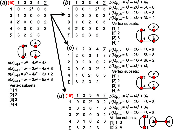
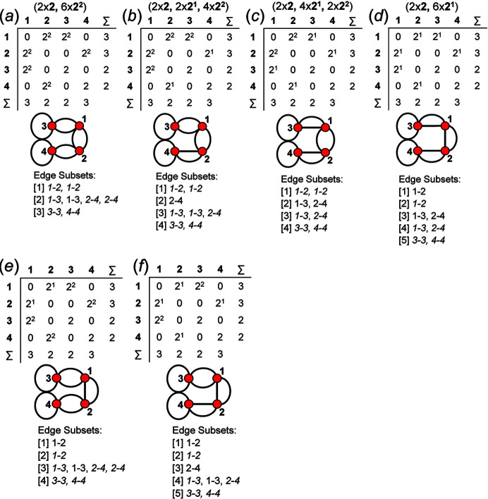
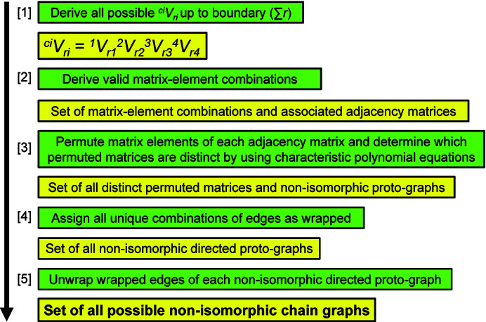
Chain, ribbon and tube silicates are based on one-dimensional polymerizations of (TO₄)^n- tetrahedra, where T = Si⁴⁺ plus P⁵⁺, V⁵⁺, As⁵⁺, Al³⁺, Fe³⁺ and B³⁺. Such polymerizations may be represented by infinite graphs (designated chain graphs) in which vertices represent tetrahedra and edges represent linkages between tetrahedra. The valence-sum rule of bond-valence theory limits the maximum degree of any vertex to 4 and the number of edges linking two vertices to 1 (corner-sharing tetrahedra). The unit cell (or repeat unit) of the chain graph generates the chain graph through action of translational symmetry operators. The (infinite) chain graph is converted into a finite graph by wrapping edges that exit the unit cell such that they link to vertices within the unit cell that are translationally equivalent to the vertices to which they link in the chain graph, and the wrapped graph preserves all topological information of the chain graph. A symbolic algebra is developed that represents the degree of each vertex in the wrapped graph. The wrapped graph is represented by its adjacency matrix which is modified to indicate the direction of wrapped edges, up (+c) or down (-c) along the direction of polymerization. The symbolic algebra is used to generate all possible vertex connectivities for graphs with ≤8 vertices. This method of representing chain graphs by finite matrices may now be inverted to generate all non-isomorphic chain graphs with ≤8 vertices for all possible vertex connectivities. MatLabR2019b code is provided for computationally intensive steps of this method and ∼3000 finite graphs (and associated adjacency matrices) and ∼1500 chain graphs are generated.

Keywords: adjacency matrix; bond topology; chain graph; edge set; graph generation; isomorphism; silicates; tetrahedra; translational symmetry; vertex set.

Figure 1

(a) A labelled graph with vertices indicated by red circles and edges indicated by black lines, (b) the vertex and edge set of the graph. Vertices 1 and 3 are of degree 3 (3-connected) and vertices 2 and 4 are of degree 2 (2-connected).

Figure 2

(a) An infinite chain graph with vertices of degree 1 and 3, in which repeat units are separated by dashed lines and edge 2–2 extends outside the repeat unit; (b) a finite wrapped graph in which edges that extend outside the repeat unit in (a) are wrapped to form a loop at vertex 2; (c) an infinite chain graph with vertices of degree 1, 2 and 3; (d) a finite wrapped graph in which edges that extend outside the repeat unit in (c) are wrapped to form a curved edge between vertices 1 and 2. Straight black arrows indicate the infinite extension of chain graphs in the +c and −c directions. Curved black arrows in (a) and (c) indicate how edges are wrapped in (b) and (d), and curved black lines represent wrapped edges in (b) and (d). Dashed black lines show the repeat units of each chain graph.

Figure 3

Two topologically distinct (non-isomorphic) chain graphs: (a) a chain graph of four-membered rings (squares), and (b) a chain graph of six-membered rings (hexagons) in which edges that extend outside the repeat unit in the +c and −c directions are shown with green and red arrows, respectively. (c), (d) The wrapped graphical representations of (a) and (b) are topologically identical (isomorphic) and differentiated by indicating the direction of wrapped (curved) edges with red and green arrows. Straight black arrows in (a) and (b) indicate the infinite extension of chain graphs in the +c and −c directions. Curved black arrows indicate how edges are wrapped in (a) and (b), and curved black lines represent wrapped edges in (c) and (d). Dashed black lines show the repeat units of each chain graph.

Figure 4

(a) Tetrahedron, (b) ball-and-stick and (c) graphical representations of the chain in astrophyllite-supergroup minerals viewed orthogonally to the c axis. Each tetrahedron in (a) is represented by a point (ball) in (b) and a vertex in (c), and all linkages between tetrahedra in (a) are represented by lines (sticks) in (b) and edges in (c) that connect each ball or vertex. Red and blue balls (points) represent 3- and 1-connected vertices, respectively. Dashed black lines show the ¹ T ₂ ³ T ₂ geometrical repeat unit (n _g) in (a) and (b), and the ¹ V ₁ ³ V ₁ topological repeat unit (n _t) in (c).

Figure 5

A chain graph with vertex connectivity ² V ₁ (red vertices and black edges) to which ¹ V ₁ vertices (green vertices and edges) have been added, forming a chain graph with vertex connectivity ¹ V ₁ ³ V ₁. The red circle indicates a vertex that has been changed from degree 2 to 3 by the connection with a 1-connected vertex. Dashed black lines show the repeat unit of the chain graph.

Figure 6

(a) A finite graph with vertex connectivity ² V ₂ ³ V ₂ ⁴ V ₁ and (b) the corresponding adjacency matrix in which each row (or column) represents a vertex and the sums of rows and columns equal the degree of the respective vertices. Cells of the upper and lower triangle are outlined in red and separated by diagonal cells.

Figure 7

(a) A chain graph with vertex connectivity ¹ V ₁ ³ V ₁, (b) the corresponding wrapped graph and (c) the corresponding adjacency matrix. (d) A chain graph with vertex connectivity ¹ V ₁ ² V ₁ ³ V ₁, (e) the corresponding wrapped graph and (f) the corresponding adjacency matrix. Curved black arrows indicate how edges are wrapped in (a) and (d), and curved black lines represent wrapped edges in (b) and (e). Coloured arrows in (b) are not required as the loop on vertex 2 represents linkage to equivalent vertices (2′ and 2′′) in the +c and −c directions. Green and red arrows in (e) and matrix-element superscripts in (f) indicate the number and direction of wrapped edges. Dashed black lines show the repeat units of each chain graph.

Figure 8

(a) A chain graph with vertex connectivity ² V ₁ ³ V ₄, (b) the corresponding wrapped graph and (c) the corresponding adjacency matrix. Curved black lines in (b) represent wrapped edges in (a); green and red arrows in (b) and matrix-element superscripts in (c) indicate the number and direction of wrapped edges. Note that it is not necessary to indicate the direction of the wrapped edges linking vertices 2 and 3. Dashed black lines show the repeat units of each chain graph.

Figure 9

The vertex connectivity, ^cV_r , of observed chain, ribbon and tube topologies as a function of ∑r for c = 1–4. Most observed topologies have ∑r ≤ 8; hence the boundary limit for graph generation has been set to ∑r = 8 and is shown by the red line. Squares indicate the ^cV_r expression and ∑r for one (yellow) and more than one (green) observed topology. [Data from Day & Hawthorne (2020 ▸).]

Figure 10

(a) A graph with vertex connectivity ² V ₂ ³ V ₂ and its corresponding adjacency matrix ([A]), (b) the reduced graph produced by removing vertex 1 from the graph in (a) and the corresponding reduced adjacency matrix ([A]−1), and (c) the characteristic polynomial equation for the reduced adjacency matrix in (b): [p(λ)_[A]−1].

Figure 11

The reduced graphs, corresponding reduced adjacency matrices, and characteristic polynomial equations after the following vertices have been removed from the graph in Fig. 10 ▸(a): (a) vertex 2, p(λ)_[A]−2, (b) vertex 3, p(λ)_[A]−3 and (c) vertex 4, p(λ)_[A]−4. (d) The original graph, adjacency matrix and the vertex subsets determined using characteristic polynomial equations.

Figure 12

All distinct adjacency matrices that produce proto-graphs with vertex connectivity ² V ₂ ³ V ₂. The matrix-element combination (4 × 1)(1 × 2)(2 × 2¹) corresponds to matrices [7] and [7′], (4 × 1)(1 × 2)(2 × 2²) corresponds to matrices [8] and [8′], (2 × 1)(2 × 2)(2 × 2¹) corresponds to matrices [10] and [10′], and (2 × 1)(2 × 2)(2 × 2²) corresponds to matrices [11] and [11′]. All other valid matrix-element combinations correspond to a single matrix.

Figure 13

All valid matrix-element combinations and their associated proto-graphs with vertex connectivity ² V ₂ ³ V ₂. The corresponding adjacency matrices are shown in Fig. 12 ▸.

Figure 14

For vertex connectivity ² V ₂ ³ V ₂, (a) the adjacency matrix [1] for the matrix-element combination (10 × 1), the corresponding proto-graph, the characteristic polynomial equations of the reduced proto-graphs and the resulting vertex subsets; (b), (c) and (d) three permutated versions of this adjacency matrix and proto-graph. The characteristic polynomial equations of the reduced adjacency matrices are identical, confirming that these adjacency matrices correspond to isomorphic proto-graphs.

Figure 15

For vertex connectivity ² V ₂ ³ V ₂, (a) adjacency matrix [7] for the matrix-element combination (4 × 1)(1 × 2)(2 × 2¹), the corresponding proto-graph, the characteristic polynomial equations of the reduced proto-graphs and the resulting vertex subsets. (b), (c), (d) Three permutated versions of this adjacency matrix and proto-graph, and the characteristic polynomial equations of the reduced adjacency matrices. The characteristic polynomial equations of the reduced adjacency matrices in (b) and (c) are identical to those in (a) (adjacency matrix [7]), confirming that the reduced proto-graphs are isomorphic. The characteristic polynomial equations for the reduced adjacency matrices derived from adjacency matrix [7′], shown in (d), are different, confirming that this proto-graph is non-isomorphic with the other proto-graphs.

Figure 16

For vertex connectivity ² V ₂ ³ V ₂, (a) adjacency matrix [10] for the matrix-element combination (2 × 1)(2 × 2)(2 × 2¹), the corresponding proto-graph, the characteristic polynomial equations of the reduced proto-graphs and the resulting vertex subsets. (b), (c), (d) Three permutated versions of this adjacency matrix and proto-graph, and the characteristic polynomial equations of the reduced adjacency matrices. The characteristic polynomial equations of the reduced adjacency matrices in (b) and (c) are identical to those in (a) (adjacency matrix [10]), confirming that these proto-graphs are isomorphic. The characteristic polynomial equations for the reduced adjacency matrices derived from adjacency matrix [10′], shown in (d), are different, confirming that this proto-graph is non-isomorphic with the proto-graphs in (b) and (c).

Figure 17

For vertex connectivity ² V ₂ ³ V ₂, (a) the proto-graph for the matrix-element combination (10 × 1), (b) the corresponding vertex subsets, (c) the corresponding edge subsets. (d) The proto-graph for the matrix-element combination (2 × 1)(4 × 2¹), (e) the corresponding vertex subsets, (f) the corresponding edge subsets.

Figure 18

The MatLabR2019b output of all possible valid matrix-element combinations and corresponding non-isomorphic proto-graphs for the vertex connectivity ⁴ V ₄.

Figure 19

For vertex connectivity ⁴ V ₄, the adjacency matrix, corresponding proto-graph and edge subsets for the matrix-element combinations (a) (2 × 2)(6 × 2²), (b) (2 × 2)(2 × 2¹)(4 × 2²), (c) (2 × 2)(4 × 2¹)(2 × 2²) and (d) (2 × 2)(6 × 2¹). The matrix-element combinations (2 × 2)(2 × 2¹)(4 × 2²) and (2 × 2)(4 × 2¹)(2 × 2²) correspond to a second distinct matrix and non-isomorphic proto-graph shown in (e) and (f), respectively. The adjacency matrices and corresponding proto-graphs in (b)–(f) are not produced by the MatLabR2019b code and must be derived manually. In edge subsets, wrapped edges are italicized.

Figure 20

For vertex connectivity ² V ₂ ³ V ₂, (a) a proto-graph for the matrix-element combination (10 × 1) and its vertex and edge subsets, (b) the directed proto-graph in which the 1–2 edge (of edge subset [2]) has been assigned as wrapped in the +c direction, and (c) the resultant chain graph. (d) The directed proto-graph in which the 2–3 edge (of edge subset [1]) has been assigned as wrapped in the +c direction, and (e) the resultant chain graph. Note how unwrapping single edges that belong to different edge subsets results in non-isomorphic chain graphs. Legend as in Fig. 7 ▸; the green and red arrows on the curved 1–2 and 2–3 edges denote the directions in which the edge is to be unwrapped: green = in the +c direction, red = in the −c direction.

Figure 21

For vertex connectivity ¹ V ₁ ³ V ₃, (a) a proto-graph for the matrix-element combination (6 × 1)(2 × 2¹) and the corresponding vertex and edge subsets, (b) the directed proto-graph in which the 3–4 edge is assigned as wrapped in the +c direction and the corresponding adjacency matrix and edge subsets, and (c) the resultant chain graph. (d) The directed proto-graph in which the 3–4 and 1–2 edges have been assigned as wrapped in the +c direction and the corresponding adjacency matrix and edge subsets, and (e) the resultant chain graph. (f) The directed proto-graph in which the 3–4 and 1–2 edges have been assigned as wrapped in the +c and −c directions, respectively, and the corresponding adjacency matrix and edge subsets, and (g) the resultant chain graph. Note that the chain graphs in (e) and (g) are isomorphic with the chain graph in (c). The blue arrows show the direction of unwrapping of the 1–2 edge in (e) the +c direction and in (g) the −c direction. All edges and vertices of a single repeat unit in each chain graph are shown in green and yellow, respectively. Legend as in Figs. 7 ▸ and 20 ▸.

Figure 22

For vertex connectivity ² V ₂ ³ V ₂, (a) a proto-graph [identical to that in Fig. 20 ▸(a)] for the matrix-element combination (10 × 1) and the corresponding vertex and edge subsets, (b) the directed proto-graph in which the 2–3 edge is assigned as wrapped in the −c direction and the corresponding adjacency matrix and edge subsets, and (c) the resultant chain graph. (d) The directed proto-graph in which the 1–2 and 1–3 edges have been assigned as wrapped in the +c direction and the 2–3 edge in the −c direction, and the corresponding adjacency matrix and edge subsets, and (e) the resultant chain graph. (f) The directed proto-graph in which the 2–3 and 1–2 edges have been assigned as wrapped in the −c direction and the 1–3 edge in the +c direction, and the corresponding adjacency matrix and edge subsets, (g) the resultant chain graph, and (h) an untangled version of this chain graph. Note that the chain graph in (e) is isomorphic with the chain graph in (c) as unwrappings involving vertex 1 in (d) are redundant. Legend as in Fig. 21 ▸.

Figure 23

For vertex connectivity ² V ₂ ³ V ₂, (a) a proto-graph [identical to that in Fig. 20 ▸(a)] and the corresponding vertex and edge subsets, (b) the directed proto-graph in which the 1–2, 1–3, 2–4 and 3–4 edges are assigned as wrapped in the +c direction and the 2–3 edge is assigned as wrapped in the −c direction, and its corresponding adjacency matrix, and (c) the resultant chain graph. (d) The directed proto-graph produced by omitting redundant unwrappings involving vertex 1 in (b), and its corresponding adjacency matrix and edge subsets, and (e) the resultant chain graph. Note that the chain graph in (e) is isomorphic with the chain graph in (c). Legend as in Figs. 7 ▸ and 21 ▸.

Figure 24

For vertex connectivity ² V ₂ ³ V ₂, (a) a proto-graph [identical to that shown in Fig. 20 ▸(a)] and the corresponding vertex and edge subsets, (b) the directed proto-graph in which the 1–2, 1–3, 2–3 and 2–4 edges are assigned as wrapped in the +c direction and the 3–4 edge is assigned as wrapped in the −c direction, its corresponding adjacency matrix and edge subsets, and (c) the resultant chain graph. (d) The directed proto-graph produced by omitting redundant unwrappings involving vertex 1 in (b), its corresponding adjacency matrix and edge subsets, and (e) the resultant chain graph. (f) The directed proto-graph produced by omitting redundant unwrappings involving vertex 3 in (b), its corresponding adjacency matrix and edge subsets, and (g) the resultant chain graph. Note that the chain graphs in (c), (e) and (g) are isomorphic. Legend as in Figs. 7 ▸ and 21 ▸.

Figure 25

For vertex connectivity ² V ₂ ³ V ₂, (a) a proto-graph [identical to that in Fig. 20 ▸(a)] and the corresponding vertex and edge subsets, (b) the directed proto-graph in which the 1–3 and 2–3 edges are assigned as wrapped in the +c direction and the 2–4 edge in the −c direction, its corresponding adjacency matrix and edge subsets, (c) the resultant chain graph, (d) an untangled version of this chain graph. (e) The directed proto-graph produced by omitting redundant unwrappings involving vertex 3 in (b), its corresponding adjacency matrix and edge subsets, and (f) the resultant chain graph which is non-isomorphic with the chain graph in (c). (g) The directed proto-graph in which the 2–4 edge is assigned as wrapped in the −c direction and the 3–4 edge is assigned as wrapped in the +c direction, its corresponding adjacency matrix and edge subsets, (h) the resultant chain graph, and (i) an untangled version of this chain graph. Note the chain graphs in (h) and (i) are isomorphic with the chain graphs in (c) and (d). Legend as in Figs. 7 ▸ and 21 ▸.

Figure 26

For vertex connectivity ³ V ₂ ⁴ V ₁, (a) a proto-graph for the matrix-element combination (4 × 1)(2 × 1)(2 × 2¹) and its vertex and edge subsets, (b) the directed proto-graph in which the 2–3 edge is assigned as wrapped in the +c direction, its corresponding adjacency matrix and edge subsets, and (c) the resultant chain graph. (d) The directed proto-graph in which the 2–3 edge is assigned as wrapped in the +c direction and the 1–2 edge is assigned as wrapped in the −c direction, and the corresponding adjacency matrix and edge subsets, and (e) the resultant chain graph. (f) The directed proto-graph in which the 2–3 and 1–2 edges are assigned as wrapped in the +c direction, its corresponding adjacency matrix and edge subsets, and (g) the resultant chain graph. (h) The directed proto-graph in which the 2–3, 1–2 and 1–3 edges are assigned as wrapped in the +c direction, its corresponding adjacency matrix and edge subsets, and (i) the resultant chain graph. Note that the chain graphs in (e) and (i) are isomorphic with the chain graph in (c) as the unwrappings involving vertex 2 in (d) are redundant and the unwrappings involving vertex 1 in (h) are redundant. Legend as in Figs. 7 ▸ and 21 ▸.

Figure 27

(a) A proto-graph and corresponding chain graph with vertex connectivity ¹ V ₃ ² V ₄ ³ V ₁ ⁴ V ₁ in which edges 3–5, 3–2, 3–7, 2–4, 5–6, 7–8 and 8–9 and vertices 2 to 9 form linear branches, and edge 1–1 and vertex 1 form the backbone chain. (b) A proto-graph and corresponding chain graph with vertex connectivity ¹ V ₂ ² V ₁ ³ V ₂ ⁴ V ₁ in which edges 3–2, 2–4, 2–5 and 5–6 and vertices 2, 4, 5 and 6 form linear branches and edges 1–1, 3–3 and 1–3 and vertices 1 and 3 form the backbone chain. (c) A proto-graph and corresponding chain graph with vertex connectivity ² V ₂ ³ V ₄ in which edges 3–2, 3–5, 2–5, 2–4, 5–6 and 4–6 and vertices 2 to 6 form polygonal branches, and edges 1–1 and vertex 1 form the backbone chain. Legend as in Fig. 7 ▸.

Figure 28

(a) A proto-graph with vertex connectivity ¹ V ₂ ² V ₁ ³ V ₂ and its corresponding adjacency matrix, and (b) the resultant chain graph in which edges 1–2, 2–3, 3–4 and 3–5 and vertices 2 to 5 form linear branches (indicated by the green ellipse). (c) A directed proto-graph in which the 3–5 edge is assigned as wrapped in the +c direction, its corresponding adjacency matrix, and (d) the resultant chain graph. (e) The directed proto-graph in which the 2–3 and 3–5 edges are assigned as wrapped in the +c direction, the corresponding adjacency matrix, and (f) the resultant chain graph. (g) The directed proto-graph in which the 1–2, 2–3 and 3–5 edges are assigned as wrapped in the +c direction, its corresponding adjacency matrix, and (h) the resultant chain graph. Note how chain graphs in (b), (d), (f) and (h) are isomorphic. Legend as in Fig. 7 ▸.

Figure 29

(a) A proto-graph with vertex connectivity ² V ₂ ³ V ₂, its corresponding adjacency matrix, and (b) the resultant chain graph in which edges 2–3, 3–4 and 2–4 and vertices 2, 3 and 4 form polygonal branches. (c) The directed proto-graph in which the 2–4 edge is assigned as wrapped in the −c direction, and (d) the resultant chain graph which does not contain branches and is non-isomorphic with the chain graph in (b). Legend as in Fig. 7 ▸.

Figure 30

A flow chart of the overall method to derive all non-isomorphic chain graphs from the complete set of possible vertex connectivities ¹ V _r1 ² V _r2 ³ V _r3 ⁴ V _r4. Green boxes denote actions and yellow boxes denote the products.

Figure 31

Range of TO _n for chain and sheet silicates. Yellow boxes show the range that is topologically possible for one- and two-dimensional polymerizations of tetrahedra, and the green boxes show the compositional ranges observed in chain- and sheet-silicate minerals. Modified from Day & Hawthorne (2020 ▸).

References

1. Blatov, V. A., Shevchenko, A. P. & Proserpio, D. M. (2014). Cryst. Growth Des. 14, 3576–3586.
1. Brown, I. D. (2016). The Chemical Bond in Inorganic Chemistry, 2nd ed. Oxford University Press.
1. Chung, S. J., Hahn, Th. & Klee, W. E. (1984). Acta Cryst. A40, 42–50.
1. Day, M. C. & Hawthorne, F. C. (2020). Miner. Mag. 84, 165–244.
1. Delgado-Friedrichs, O. & O’Keeffe, M. (2003). Acta Cryst. A59, 351–360. - PubMed