Resolving and Predicting Neighborhood Vulnerability to Urban Heat and Air Pollution: Insights From a Pilot Project of Community Science

Abstract

Urban heat and air pollution, two environmental threats to urban residents, are studied via a community science project in Los Angeles, CA, USA. The data collected, for the first time, by community members, reveal the significance of both the large spatiotemporal variations of and the covariations between 2 m air temperature (2mT) and ozone (O₃) concentration within the (4 km) neighborhood scale. This neighborhood variation was not exhibited in either daily satellite observations or operational model predictions, which makes the assessment of community health risks a challenge. Overall, the 2mT is much better predicted than O₃ by the weather and research forecast model with atmospheric chemistry (WRF-Chem). For O₃, diurnal variation is better predicted by WRF-Chem than spatial variation (i.e., underestimated by 50%). However, both WRF-chem and the surface observation show the overall consistency in describing statistically significant covariations between O₃ and 2mT. In contrast, satellite-based land surface temperature at 1 km resolution is insufficient to capture air temperature variations at the neighborhood scale. Community engagement is augmented with interactive maps and apps that show the predictions in near real time and reveals the potential of green canopy to reduce air temperature and ozone; but different tree types and sizes may lead to different impacts on air temperature, which is not resolved by the WRF-Chem. These findings highlight the need for community science engagement to reveal otherwise impossible insights for models, observations, and real-time dissemination to understand, predict, and ultimately mitigate, urban neighborhood vulnerability to heat and air pollution.

Keywords: air quality prediction; community science and engagement; environment and public health; neighborhood scale variation; temperature and ozone; urban heat and air pollution.

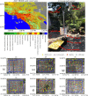
Figure 1

(a) Moderate Resolution Imaging Spectroradiometer (MODIS) land surface cover type. (b) A picture of an in‐house‐built air‐O₃ sensor node showing the assembly of multiple sensors to measure wind (by anemometers), temperature, relative humidity and pressure (by sensors in air unit), O₃ concentration (by O₃ analyzer) in the air, all at 2 m above the surface, as well as soil moisture (by soil unit). (c–g) Show the satellite view of each quadrat. The blue rectangle shows the 4 × 4 km² WRF‐Chem model grid box that collocates with each quadrat. Also denoted in (b)–(g) are the locations of iButton sensors (in yellow dots), the air‐O₃ sensor node (purple), and the MODIS 1 × 1 km² land surface temperature pixels (red) within corresponding weather and research forecast‐Chem grid box (blue square).

Figure 2

(a) A flowchart illustration and examples of citizen science engagement. Please see the text for details. (b) A series of iPhone screenshots showing the Earth System Modeling Complex app that provides citizen access to a wide range of information including the forecast for the next 3 days (first panel on the left), a map of predicted weather (second), an interactive map (third), and a detailed forecast.

Figure 3

An example showing the impacts of different type of trees on diurnal variation of temperature.

Figure 4

Impacts of canopy radius on daytime detrend temperature. Here, detrend is done by subtracting weekly moving average temperature from the measured temperature at each corresponding location.

Figure 5

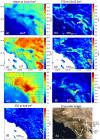
Spatial distribution of weather and research forecast model with atmospheric chemistry forecasts of (a) surface O₃ and (c) air temperature, as well as (e) Moderate Resolution Imaging Spectroradiometer (MODIS) land surface temperature (LST), averaged at 19:00 UTC in July 2017. Also shown are the evaluation of forecast parameters for each day with (b) measured O₃ concentration and (d) measured air temperature. The MODIS LST is also evaluated with 2 m air temperature (2mT) because there is no direction measurement of LST. Statistics of evaluation including the linear correlation coefficient R, the best‐fit equation, statistical significance, the mean and standard deviation of the x and y variables, and the number of data points are also shown in each evaluation panel.

Figure 6

Spatial distribution of (a) weather and research forecast model with atmospheric chemistry (WRF‐Chem) forecast of 2mT and (b) its standard deviation (STD), averaged at 19:00 UTC in July 2017 at the spatial resolution of 12 × 12 km² (e.g., 3 × 3 WRF‐Chem 4 × 4 km² grid boxes in the inner most domain). Panels (c and d) are similar to panels (a and b), respectively, but for MODIS LST; (e) and (f) are for WRF‐Chem forecasts of O₃. Also shown are (g): the Moderate Resolution Imaging Spectroradiometer land surface temperature (MODIS LST) standard deviation computed at 4 × 4 km² by using MODIS LST at 1 × 1 km² resolution, and (h) a true‐color image of the study region with different location marked (see details in the text).

Figure 7

Time series of the standard deviation of daily O₃ (left) and 2mT (right) measured by sensors in each quadrat pair and simulated by weather and research forecast model with atmospheric chemistry (at 4 × 4 km² each). See text for details.

Figure 8

(a) Scatter plot of hourly temperature and O₃ observed (yellow dot) and predicted (green dot) at each quadrat. (b) Monthly mean hourly variation of O₃ from observations and predictions as a function of local hour. (c) Is the same as (b) but for temperature. (d) Scatter plot of the measured and modeled O₃ standard deviation at each hour. (e) Is the same as (d), but for temperature.

References

1. Cabaraban, M. T. , Kroll, C. N. , Hirabayashi, S. , & Nowak, D. J. (2013). Modeling of air pollutant removal by dry deposition to urban trees using a WRF/CMAQ/i‐tree eco coupled system. Environmental Pollution, 176, 123–133. 10.1016/j.envpol.2013.01.006 - DOI - PubMed
1. Chambers, L. H. , McKeown, M. A. , McCrea, S. A. , Martin, A. M. , Rogerson, T. M. , & Bedka, K. M. (2017). CERES S’COOL project update: The evolution and value of a long‐running education project with a foundation in NASA Earth science missions. Bulletin of the American Meteorological Society, 98(3), 473–483. 10.1175/bams-d-15-00248.1 - DOI - PMC - PubMed
1. Churkina, G. , Grote, R. , Butler, T. M. , & Lawrence, M. (2015). Natural selection? Picking the right trees for urban greening. Environmental Science & Policy, 47, 12–17. 10.1016/j.envsci.2014.10.014 - DOI
1. Elmore, K. L. , Flamig, Z. L. , Lakshmanan, V. , Kaney, B. T. , Farmer, V. , Reeves, H. D. , & Rothfusz, L. P. (2014). MPING: Crowd‐sourcing weather reports for research. Bulletin of the American Meteorological Society, 95(9), 1335–1342. 10.1175/bams-d-13-00014.1 - DOI
1. Escobedo, F. J. , & Nowak, D. J. (2009). Spatial heterogeneity and air pollution removal by an urban forest. Landscape and Urban Planning, 90(3), 102–110. 10.1016/j.landurbplan.2008.10.021 - DOI
LinkOut - more resources