Using positional information to provide context for biological image analysis with MorphoGraphX 2.0

Abstract

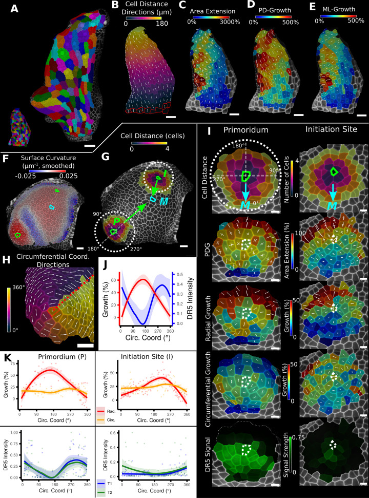
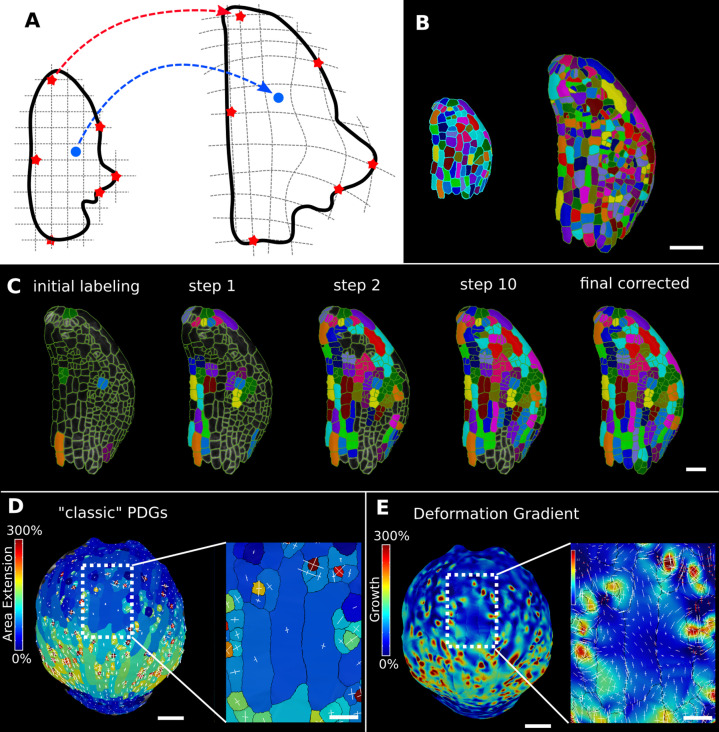
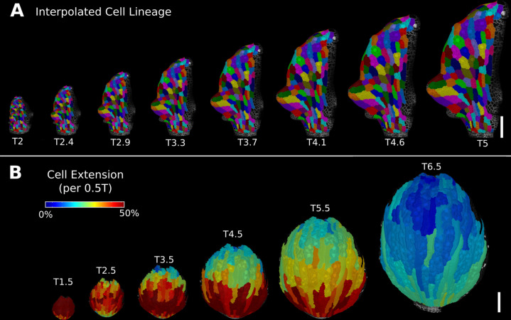
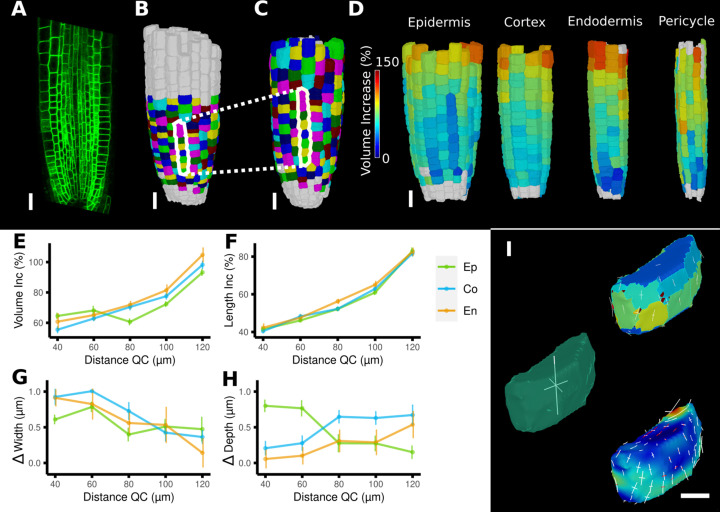
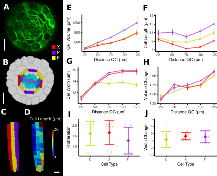
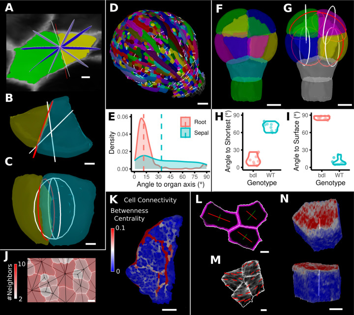
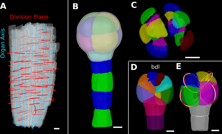
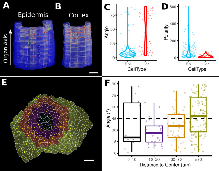
Positional information is a central concept in developmental biology. In developing organs, positional information can be idealized as a local coordinate system that arises from morphogen gradients controlled by organizers at key locations. This offers a plausible mechanism for the integration of the molecular networks operating in individual cells into the spatially coordinated multicellular responses necessary for the organization of emergent forms. Understanding how positional cues guide morphogenesis requires the quantification of gene expression and growth dynamics in the context of their underlying coordinate systems. Here, we present recent advances in the MorphoGraphX software (Barbier de Reuille et al., 2015⁠) that implement a generalized framework to annotate developing organs with local coordinate systems. These coordinate systems introduce an organ-centric spatial context to microscopy data, allowing gene expression and growth to be quantified and compared in the context of the positional information thought to control them.

Keywords: A. thaliana; convolutional neural networks; developmental biology; morphogenesis; plant biology; positional information; quantification; segmentation.

Figure 1.. Cellular segmentation and basic quantifications supported by MorphoGraphX demonstrated by using a time-lapse series of an A. thaliana flower meristem.

(A) Multichannel confocal microscopy images with a cell wall signal (red) and DR5 marker signal (green). Shown are the last three time points (T1–T3) of a four-image series (T0–T3). (B, C) Extracted surface mesh of T2. Cell wall signal near the surface was projected onto the curved mesh to enable the creation of the cellular segmentation in (C). The segmented meshes provide the base for further analysis within MorphoGraphX as shown in (D) and (E). (D) Top: MorphoGraphX allows the quantification of cellular properties such as cell area and shape anisotropy (shown as heat maps). The white axes show the max and min axes of the cells. Bottom: heat map of the quantification of the DR5 marker signal (arbitrary units) projected onto the cell surface mesh. (E) When cell lineages are known, time-lapse data can be analyzed. Top: heat maps of cell area expansion and growth anisotropy (computed from T1 to T2). The white crosses inside the cells depict the principal directions of growth. Bottom: visualization of the cell lineages and heat map of cellular proliferation (number of daughter cells), computed from T0 to T2. Scale bars: (A) 50 μm; (B– E) 20 μm. See also user guide Chapters 1–15 and tutorial videos S1 and S2 videos S1 and S2available at https://doi.org/10.5061/dryad.m905qfv1r.

Figure 1—figure supplement 1.. Basic 3D analysis using MorphoGraphX demonstrated using an Arabidopsis ovule.

(A) Confocal microscopy image with cell wall staining. (B) Segmented mesh with volumetric cells. (C) The segmented mesh allows cellular geometry to be quantified. Shown is a heat map of cell volumes. Scale bar: 50 μm. See also user guide Chapters 20–21 and tutorial video S6 available at https://doi.org/10.5061/dryad.m905qfv1r.

Figure 2.. Methods to define positional information and their application to data analysis in plant organs.

(A) Y-axis aligned A. thaliana root. The cells are colored according to the y-coordinate of their centroid position. (B) Plot of cell volumes of epidermis cells of the root in (A) along the y-axis with a fitted trend line. (C) Seedling of A. thaliana with a surface segmentation of the epidermis. A manually defined Bezier curve (white) allows the assignment of accurate cell coordinates along a curved organ axis. (D) Side and top views of an A. thaliana sepal with a proximal-distal (PD) axis heat coloring. The cell coordinates were assigned by computing the distance to manually selected cells (outlined in red) at the organ base. This method allows organ coordinates to be assigned in highly curved tissues. (E) Side and top views of (D) with a heat map coloring based on cellular growth to the next time point. (F) Plot summarizing the growth data of (E) using the PD-axis coordinates from (D). See Figure 2—figure supplement 1 for the analysis of the complete time-lapse series. Scale bars: (A) 20 μm; (C) 100 μm; (D, E) 50 μm. See also user guide Chapter 23 ‘Organ-centric coordinate systems’ and tutorial video S3video S3 available at https://doi.org/10.5061/dryad.m905qfv1r.

Figure 2—figure supplement 1.. From cellular resolution heat maps to a global analysis of A. thaliana sepal development using organ-centric coordinates.

(A, B) Heat maps of cell area extension (A) and cell proliferation (B) for each time point (visualized on the earlier point). (C) Plot of the heat map data from (A) vs. the distance of cells to the base of the organ (see also Figure 2D). The distance of the maximum of the growth zone from the base or the organ is relatively constant. However, organ length increases about 10× between the first and last time points, making a comparison of the different curves difficult. (D–F) When plotting the same data with normalized cell distance values averaged using 20 bins along the proximal-distal axis, it becomes more apparent that the growth zone moves from the proximal to the distal regions over the course of development (D). The trend of lower and more proximal maxima (highlighted with arrows) is even clearer when proliferation is plotted in the same way (E). (F) Cell area data plotted as in (D) and (E). Average cell areas increase mainly at the distal end during later time points. Scale bars: (A, B) 100 μm.

Figure 3.. Examples of data analyses using organ coordinate directions.

(A–E) Quantification of cellular growth along organ axes in a young A. thaliana leaf. (A) Segmented meshes of the leaf primordium at 3 and 6 days after initiation shown with cell labels and lineages of the earlier time point (3 days). (B) Earlier time point of (A) with proximal-distal (PD) axis coordinates (heat map) and directions (white lines) computed from selected cells at the leaf base. (C) Area extension (heat map) and principal directions of growth (PDGs, white lines) between the time points of (A). PDG axes are computed per cell and can point in different directions. (D, E) Computation of the growth component of (C) that is directed along the PD and the orthogonal medial-lateral (ML) axis. (F–K) Quantification of locally directed growth in leaf primordium and initiation site of a tomato meristem. (F) Smoothed heat map of cell curvature. Local maxima in this heat map (green and cyan cells) were selected as meristem center (M), primordium center (P), and initiation site (I) as shown in (G). (H) To analyze the data, we defined circumferential coordinate systems with their axes directions (white lines) around the primordium and initiation center (not shown), and aligned them towards the meristem center. (I) Heat maps of cell distance, area extension, radial and circumferential growth, and normalized DR5 signal intensity of the aligned primordium and initiation site. (J) Plotting the data of (I) reveals a negative correlation of the DR5 signal intensity and radial growth around the developing primordium. (K) Detailed plots of radial (red) and circumferential growth (orange) as well as the normalized DR5 signal intensity of the primordium and initiation site. Scale bars: (A) 50 μm; (B–H) 20 μm; (I) 10 μm. See also user guide Chapters 16 ‘Custom axis directions,’ 23 ‘Organ-centric coordinate systems,’ and tutorial video S3 available at https://doi.org/10.5061/dryad.m905qfv1r.

Figure 4.. Methods to create organ coordinates for 3D meshes and label different cell types.

(A–D) Organ coordinates and cell types for volumetric meshes. (A) Heat map of the surface distance for cell centroids in an A. thaliana shoot apical meristem. (B) For volumetric tissues, often a single direction is not enough to capture the geometry of the organ. Different methods can be combined such as a Bezier curve (white dashed line) with a surface mesh (gray) to create a heat map of the relative radial distance of cells in the A. thaliana root. (C, D) Organ coordinates can be used to assign cell-type labels as demonstrated in the 3D Cell Atlas plug-in for meristem and root. See also Figure 4—figure supplement 1. (E–H) Different methods to create cell-type labelings. (E) A. thaliana gynoecium (fruit epidermis) surface segmentation with a heat map of the length of the minor cell axis as obtained from a principal component analysis (PCA) on the cells’ triangles. The heat values can be thresholded to assign two cell types. (F) The same principle can be used on organ coordinates that results in a clean separation of replum (green) and valve tissue (blue). (G) We generalized the 2D clustering approach of 3D Cell Atlas (see Figure 4—figure supplement 1) so that it can be used for any measure pair and on subset selections of cells. Shown is a 2D plot of the minor axis length (x-coord) and cell signal intensity (y-coord) on the valve tissue in (F). Manually assigning clusters can separate the stomata, which are typically smaller with higher signal values (yellow) and the remaining valve cells (blue) efficiently. See also Figure 4—figure supplement 1 for 2D plots of all cells. (H) The support vector machine (SVM) classification is able to separate the three shown cell types in a higher dimensional space by using a variety of different measures and a relatively small training set. Scale bars: (A–D) 20 μm; (E–H) 50 μm. See also user guide Chapter 24 ‘Cell atlas and cell type classification’ and tutorial videos S3 and S4 available at https://doi.org/10.5061/dryad.m905qfv1r.

Figure 4—figure supplement 1.. Cell-type labeling methods and their use in the data analysis.

(A–C) Methods supported by the 3D Cell Atlas add-on demonstrated on a A. thaliana root (Montenegro-Johnson et al., 2015). (A) Longitudinal cross section with a heat map of circumferential cell size. The white dashed line is the manually defined central axis. (B) The 2D heat plot of radial distance (heat map: in Figure 4B) and circumferential cell size (heat map in A) reveals a distinct clustering and can be used directly to assign the different cell types (dashed ellipses). (C) Final result of the cell-type assignment. (D) The 3D Cell Atlas meristem (Montenegro-Johnson et al., 2019)⁠ allows the assignment of cell layers (as also seen in Figure 4C) and types in the meristem. (E–G) Cell-type-specific data analysis on the example of the A. thaliana gynoecium (Figure 4E–H). (E) Violin plot of the rectangularity of different cell types. Valve tissue cells are less rectangular and have higher variance compared to replum cells and stomata. (F, G) 2D scatter plots with fitting ellipses. Choosing different measures as x- or y-axis allows the separation of different cell types as demonstrated in Figure 4G. Scale bars: (A, C, D) 20 μm.

Figure 5.. Quantification of volumetric cell sizes along organ axes in the outer layer of the outer integument of an A. thaliana ovule.

(A) Extraction of cell layer of interest (colored in green) using an organ surface mesh. (B) Selection of the central cell file (in red) with cell distance heat map to exclude lateral cells (heat values >40 µm). (C) The centroids of the selected cells from (B) were used to specify a Bezier curve defining the highly curved organ axis from the proximal to the distal side. Heat coloring of the cells according to their coordinate along the Bezier. (D–F) Analysis of the cellular geometry in 3D. (D) Heat map of cell volume and the tensor of the three principal cell axes obtained from a principal component analysis on the segmented stack. (E) Bezier directions and associated cell length. (F) Directions perpendicular to the surface and associated cell depth. (G) Plots of the various cellular parameters relative to the Bezier coordinate. A few small cells at the distal tip of the integuments were removed from the analysis. Scale bars: 20 μm. See also user guide Chapters 21–24 and tutorial video S3 available at https://doi.org/10.5061/dryad.m905qfv1r.

Figure 6.. Deformation functions in MorphoGraphX.

(A) Deformation functions allow a direct mapping of arbitrary points (blue) between two meshes. They require the definition of common landmarks (red stars). (B, C) Semi-automatic parent labeling using deformation functions. (B) Two consecutive time points of an A. thaliana leaf primordium segmented into cells. (C) The automatic parent labeling function requires the definition of a few manually labeled cells as initial landmarks. From this sparse correspondence, a mapping between the meshes can be created and new cell associations between the two meshes are added and checked for plausibility. With more cells found, the mapping between the meshes is improved for the next iteration. (D, E) Comparison of the classic principal directions of growth (PDGs) in (D) with the gradient of a deformation function computed using the cell junctions from a complete cell lineage in (E) on an A. thaliana sepal. The classic PDGs compute a deformation for each cell individually and are shown with a heat map of areal extension for each cell. In contrast, the deformation function is a continuous function on the entire mesh. Here, heat values are derived by multiplying the amount of max and min growth. Using the deformation function gradient subcellular growth patterns that were previously hidden are revealed, such as differential growth within a single giant cell. Scale bars: (B, D, E) 50 μm; (C and zoomed regions in D and E) 20 μm. See also user guide Chapter 17 ‘Mesh deformation and growth animation’ and tutorial videos S1 and S2 available at https://doi.org/10.5061/dryad.m905qfv1r.

Figure 6—figure supplement 1.. Deformation functions allow the interpolation of intermediate steps that can be turned into a continuous sequence or animation.

(A) Animation of the early leaf development of A. thaliana created from T2 and T5 of Figure 5, shown with the lineages of T2. (B) Intermediate stages of the animation of the sepal growth of A. thaliana. For the actual time points, see Figure 2—figure supplement 1. Scale bars: 100 μm. See also user guide Chapter 17 ‘Mesh deformation and growth animation’” and tutorial video S5 available at https://doi.org/10.5061/dryad.m905qfv1r.

Figure 7.. Time-lapse analysis and visualization of 3D meshes.

(A) Cross section of the confocal stack of the first time point of a live imaged A. thaliana root. (B, C) The 3D segmentations of two time points imaged 6 hr apart. Shown are the cell lineages that were generated using the semi-automatic procedure following a manual correction. (D) Exploded view of the second time point with cells separated by cell types (see also Figure 4D). Cells are heat colored by their volume increase between the two time points. (E–H) Quantification of cellular growth along different directions within the organ. (E) Plot of the heat map data of (D). The cellular data was binned based on the distance of cells from the quiescent center (QC). Shown are mean values and standard deviations per bin. (F–H) Similarly binned data plots of the change in cell length (F), width (G), and depth (H). It can be seen that the majority of growth results from an increase in cell length. See Figure 7—figure supplement 1 for a detailed analysis of the cells in the endodermis. (I) Different ways to visualize 3D growth demonstrated using a single cortex cell: principal directions of growth (PDGs) averaged over the entire cell volume (left), PDGs averaged over the cell walls projected onto the walls (top right), and subcellular vertex-level PDGs projected onto the cell walls (bottom right). Scale bars: (A–D) 20 μm; (I) 5 μm. See also user guide Chapter 21 ‘Mesh 3D analysis and quantification’ and tutorial videos S6 and S7 available at https://doi.org/10.5061/dryad.m905qfv1r.

Figure 7—figure supplement 1.. Time-lapse analysis of cellular geometry in the A. thaliana root endodermis.

(A) Cross section of the confocal image of time point 1. (B) Segmentation with extended cell-type labeling in the endodermis. The root cell-type labeling of Figure 4D was extended by identifying the xylem cells (light purple) in the stele (cyan), their adjacent pericycle cells (blue), and assigned the endodermis cells neighboring those pericycle cells as xylem file cells (X, red). Then the endodermis cells at right angles to the xylem files were assigned phloem file (P, purple) and the remaining other endodermis cells (E, yellow). (C) Side view of one cell file of each cell type. As the cell types do not change along the cell file, it was possible to automatically assign the cell files based on their circumferential coordinate. (D) Cell files of (C) with a heat map of cell length indicating smaller cells in the xylem pole. (E–J) Quantifications of cell geometry and development in the endodermis cell types. Cellular data was binned according to their distance from the quiescent center (QC) (E–H). Shown are mean values and standard deviations per bin (E–H) or cell type (I, J). Phloem file cells showed a larger volume (E), which was caused by a greater cell length (F), an observation that has been made before by Andersen et al., 2018. In contrast, xylem file and other endodermis cells were smaller in volume due to different reasons: while xylem file cells were the shortest (E), rest endodermis cells showed a lower cell width with increasing distance from the QC (G). The time-lapse analysis confirmed above observations: while volume change was similar across the cell types (H), phloem file cells showed a lower proliferation rate (I), whereas rest endodermis cells showed the smallest extension of cell width (J). Scale bars: (A, B) 20 μm; (C, D) 50 μm.

Figure 8.. Advanced data analysis and visualization tools.

(A) Division analysis of a cell from a surface segmentation of an A. thaliana sepal. A planar approximation of the actual plane is shown in red and other potential division planes in white/blue. The actual wall is very close to the globally shortest plane. (B, C) Top and side views of a recently divided 3D segmented cell. The daughter cells are colored yellow and cyan. The red circle depicts the flat approximation plane of the actual division wall. The two white rings depict the two smallest area division planes found by simulating divisions through the cell centroid of the mother cell (i.e., the combined daughter cells). (D) Visualization of the actual planes (white lines) between cells that divided into two daughter cells in the A. thaliana sepal. (E) Density distribution and median (dashed line) of the angle between the division plane and the primary organ axis in sepal (see D) and root (see Figure 8—figure supplement 1A). The division in sepals is less aligned with the organ axis. (F) Half of an A. thaliana wildtype embryo in the 16-cell stage. This view shows that the divisions leading to this stage are precisely regulated to form two distinct layers in the embryo. (G) A visualization of the actual planes (red circles) and the shortest planes (white circles) in the wild type. Cells are colored according to the label of the mother cells. (H, I) Violin plots of quantifications of the planes show that the wild type does not follow the shortest wall rule unlike the auxin-insensitive-inducible bdl line RPS5A>>bdl. The bdl divisions are almost orthogonal to the organ surface (see Figure 8—figure supplement 1B, D, E), whereas the wild type divides parallel to the surface. Consequently, the bdl fails to form a distinct inner layer. (J, K) Cellular connectivity network analysis. (J) Cell connectivity network analysis on a young A. thaliana leaf. Cells are heat colored based on the number of neighbors, edges in the cell connectivity graph are shown in black. (K) Heat map of betweenness centrality. The betweenness reveals pathways that might be of importance for information flow, potentially via the transport of auxin. (L–N) Cell-based signal analysis. (L) Analysis of cell polarization on a surface mesh. (M) Microtubule signal analysis on a surface mesh. (N) Top and side views of a cell polarization analysis on a volumetric mesh (root epidermis PIN2, see Figure 8—figure supplement 2A–D for details). Scale bars: (A, B, C, L, M) 2 μm; (D) 50 μm; (F, G, J, N) 5 μm; (K) 100 μm. See also user guide Chapter 25 ‘Cell division analysis.’, Chapter 18 'Quantifying signal orientation', and Chapter 21.7 'Signal orientation for 3D meshes'.

Figure 8—figure supplement 1.. Details of the cell division analysis examples from Figure 8.

(A) Second time point of an A. thaliana root (see Figure 7C) that was used for the division plane analysis in Figure 8E. Cells are shown semi-transparently (gray) with their longitudinal organ axis (cyan) obtained from the analysis using 3D Cell Atlas in Figure 4B. Planar approximations of the division planes between cells that divided between the two time points are shown as red circles. Consistent with the quantitative analysis in Figure 8E, most planes are aligned with the organ axis. (B, C) A. thaliana wildtype embryo at the 16-cell stage segmented into volumetric cells shown with an organ surface mesh (gray, semi-transparent, B) and shown in an exploded view (C) to enable the visualization and access of inner layers. (D, E) Corresponding panels to Figure 8F and G for bdl embryo. Scale bars: (A–C) 10 μm; (D, E) 5 μm.

Figure 8—figure supplement 2.. Example analyses of cell polarity and microtubule signals of the data shown in Figure 8M and N.

(A–D) Quantification of PIN2 polarity in volumetric cells of an A. thaliana root. (A, B) Heat map of PIN2 concentration on epidermis and cortex. Green lines depict directionality and strength of the PIN2 concentration. (C, D) Violin plots of the orientation data for division planes and PIN2 polarity for epidermis and cortex cells. Epidermis cells show considerably stronger polarity (D) and are more aligned with the (longitudinal) organ axis (C). (E, F) Microtubule analysis on a shoot apical meristem (SAM) of A. thaliana. (E) The cells on the SAM were binned according to their distance to the SAM center. Cells are heat colored according to their bin. Yellow lines show the direction and strength of the microtubule orientation. (F) Boxplot of the angular difference between microtubule orientation and the circumferential direction around the center of the SAM (similar to Figure 5H). Scale bars: (A, B) 20 μm; (E) 10 μm. See also user guide Chapter 18 ‘Quantifying signal orientation.’ and Chapter 21.7 'Signal orientation for 3D meshes'.

References

1. Aegerter-Wilmsen T, Heimlicher MB, Smith AC, de Reuille PB, Smith RS, Aegerter CM, Basler K. Integrating force-sensing and signaling pathways in a model for the regulation of wing imaginal disc size. Development (Cambridge, England) 2012;139:3221–3231. doi: 10.1242/dev.082800. - DOI - PubMed
1. Andersen TG, Naseer S, Ursache R, Wybouw B, Smet W, De Rybel B, Vermeer JEM, Geldner N. Diffusible repression of cytokinin signalling produces endodermal symmetry and passage cells. Nature. 2018;555:529–533. doi: 10.1038/nature25976. - DOI - PMC - PubMed
1. Armour WJ, Barton DA, Law AMK, Overall RL. Differential Growth in Periclinal and Anticlinal Walls during Lobe Formation in Arabidopsis Cotyledon Pavement Cells. The Plant Cell. 2015;27:2484–2500. doi: 10.1105/tpc.114.126664. - DOI - PMC - PubMed
1. Barbier de Reuille P, Routier-Kierzkowska AL, Kierzkowski D, Bassel GW, Schüpbach T, Tauriello G, Bajpai N, Strauss S, Weber A, Kiss A, Burian A, Hofhuis H, Sapala A, Lipowczan M, Heimlicher MB, Robinson S, Bayer EM, Basler K, Koumoutsakos P, Roeder AHK, Aegerter-Wilmsen T, Nakayama N, Tsiantis M, Hay A, Kwiatkowska D, Xenarios I, Kuhlemeier C, Smith RS. MorphoGraphX: A platform for quantifying morphogenesis in 4D. eLife. 2015;4:e05864. doi: 10.7554/eLife.05864. - DOI - PMC - PubMed
1. Barkoulas M, Hay A, Kougioumoutzi E, Tsiantis M. A developmental framework for dissected leaf formation in the Arabidopsis relative Cardamine hirsuta. Nature Genetics. 2008;40:1136–1141. doi: 10.1038/ng.189. - DOI - PubMed
Publication types