ON/OFF domains shape receptive field structure in mouse visual cortex

Abstract

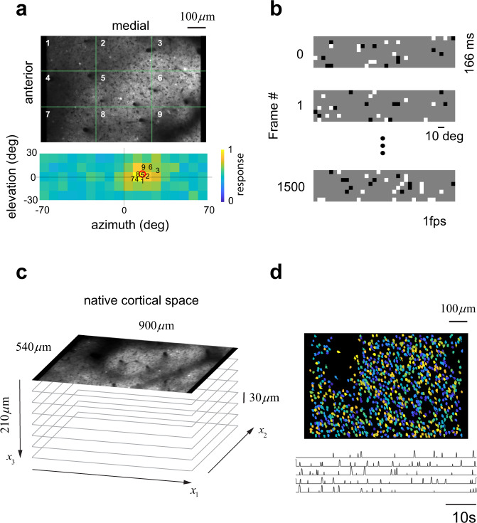
In higher mammals, thalamic afferents to primary visual cortex (area V1) segregate according to their responses to increases (ON) or decreases (OFF) in luminance. This organization induces columnar, ON/OFF domains postulated to provide a scaffold for the emergence of orientation tuning. To further test this idea, we asked whether ON/OFF domains exist in mouse V1. Here we show that mouse V1 is indeed parceled into ON/OFF domains. Interestingly, fluctuations in the relative density of ON/OFF neurons on the cortical surface mirror fluctuations in the relative density of ON/OFF receptive field centers on the visual field. Moreover, the local diversity of cortical receptive fields is explained by a model in which neurons linearly combine a small number of ON and OFF signals available in their cortical neighborhoods. These findings suggest that ON/OFF domains originate in fluctuations of the balance between ON/OFF responses across the visual field which, in turn, shapes the structure of cortical receptive fields.

Fig. 1. Basic methods.

a Coarse retinotopic mapping. The average signal originating from nine sectors defined by a 3 × 3 grid on the field of view of the microscope were used to map the aggregate receptive field and determine its center. The image at the bottom shows the location of the centers for each sector superimposed on top of the aggregate receptive field for the entire population (normalized to its peak). b Sparse-noise stimulus. Images were flashed for 166 ms and presented at a rate of 1 per second on a wide field screen. c Volumetric sampling in primary visual cortex (see Methods for details on the volumes for each experiment). d Segmentation of regions of interest (ROIs) and five sample traces showing spike inference from calcium signals. For visualization, ROIs are assigned random colors.

Fig. 2. Calculation of ON/OFF kernels and domains.

a Example of a spatio-temporal ON kernel. The panels show the correlation between the response of a neuron and the location of the presentation of bright stimuli across the visual field for different delay times between stimulus and response. The peak response, as measured by the norm of the kernel, occurs 4 frames (260 ms) after stimulus onset. Kernel is normalized between zero and one. b Raw receptive field measurements (left panels) and their Gaussian fits (right panels). Top, Cell with only a significant ON kernel. Middle, a complex cell with largely overlapping ON and OFF kernel. Bottom, a simple cell with spatially displaced ON and OFF kernels. ON and OFF kernels are normalized jointly to the absolute value attained by either of them, thus the colormap ranges from 0 to 1 and the colormap in panel a applies. In the case of ON-OFF difference maps, we normalized by the maximum absolute value of the map, thus the colormap ranges from −1 to +1. c Distribution of normalized distance in V1 neurons with significant ON and OFF maps in n = 4430 neurons pooled across all experiments. Normalized distance is defined as the distance between receptive field centers divided by the average sigma of the Gaussian fit. We define simple cells as those with a normalized distance larger than one half. d Demonstration of ON/OFF domains in native cortical space. The image on the left shows the distribution of ON cells on the cortical surface (we are projecting depth away) along with a pseudo-colormap showing the estimated density. The density estimation for OFF cells appears in the middle panel. Note that both densities appear to peak at different locations. Blue circles show two peak locations for the density of OFF cells. The red circle shows a peak location for ON cells. ON/OFF domains are evident in the difference of the densities, as shown in the right image. Level sets depict areas where the fluctuations exceed what might be expected by chance at a 0.001 level by randomly shuffling the ON/OFF labels of the cells (without changing their positions). Source data provided for panel c.

Fig. 3. A biased-input model of ON/OFF domains.

a The cartoon depicts a 1D version of the biased-input model. The bottom layer shows the location and polarities of ON/OFF cells in the visual field (ON=red, OFF=blue). The top layer shows the input of those signals into the cortex assuming an accurate retinotopy. Here, we readily see that fluctuations in the relative density of ON and OFF cells ought to follow a corresponding fluctuation in the density of ON and OFF receptive field locations in the visual field. Thus, ON/OFF domains could arise from a property of the input. Thalamic projections, of course, include axonal arborizations that are not depicted in this diagram to avoid clutter. b The cartoon represents a top view from the cortex of a set of geniculate ON and OFF-center inputs dominating the representation in different parts of the visual field. We assume an accurate retinotopy, so the spatial distribution of ON/OFF receptive fields also represents the distribution of ON/OFF afferents into the cortex. We hypothesize that clusters of ON inputs establish cortical ON domains, and clusters of OFF inputs define OFF domains. Dashed circles represent neighborhoods over which three different cortical cells can sample the geniculate inputs. Such areas are determined by the extent of thalamic arborizations and the size of cortical dendritic trees. Cortical cells with access just to (a) OFF or (b) ON inputs will develop mono-contrast receptive fields with a single subregion of the corresponding polarity. Cortical cells with access to both types of signals (c) can develop receptive fields with two subregions (three possible examples are illustrated).

Fig. 4. Alignment of cortical and visual space via canonical correlation analysis.

a, b Distribution of ON (red) and OFF (blue) neurons in the native cortical and visual spaces ($n_{\mathrm{on}}=317$, $n_{\mathrm{off}}=1178$). Native cortical space has an x₃ component that comes out of the page, so here the data are projected into the $\left(x_1,x_2\right)$ plane ignoring depth. c, d Same data as in a, b now represented in canonical cortical and visual spaces. Note how the locations a, b, c, d, corresponding to the corners of the imaging plane, are mapped to canonical visual space. A location dominated by OFF cells in cortical or visual space (a, b asterisks) will map to a location dominated by OFF cells in canonical cortical or canonical visual space (c, d asterisks). e Correlation between the first pair of canonical variables ${\widehat{x}}_1$ and ${\widehat{y}}_1$ and f the second pair ${\widehat{x}}_2$ and ${\widehat{y}}_2$. Source data provided for all panels.

Fig. 5. Correlation between ON/OFF domains and fluctuations in the balance of ON/OFF representation at the input.

Each panel displays the result of one experiment. In each case, the top row displays the density of ON ($f_{\mathrm{on}}^x$) and OFF ($f_{\mathrm{off}}^x$) cells in canonical cortical space, along with their difference, $f_{\mathrm{on}}^x-f_{\mathrm{off}}^x$. The bottom row shows the density in the position of receptive field centers for ON ($f_{\mathrm{on}}^y$) and OFF ($f_{\mathrm{off}}^y$) cells in canonical visual space, along with their difference, $f_{\mathrm{on}}^y-f_{\mathrm{off}}^y$. In all panels, both axes span the range from −2.5 to 2.5. Level sets showing areas where fluctuations are above or below the expected at the p = 0.001 significance level are shown by red and blue solid curves (Monte Carlo simulations with random shuffling of the ON/OFF labels in the population). The correlation coefficient between the fluctuations $f_{\mathrm{on}}^x-f_{\mathrm{off}}^x$ and $f_{\mathrm{on}}^y-f_{\mathrm{off}}^y$ is shown at the inset along with the statistical significance reached in each case (N = 1000 Monte Carlo simulations with reshuffling of ON/OFF labels). In each panel, the distributions are normalized by their maximum value and the colormap ranges from 0 to 1 (bottom left), while the differences of the distributions are shown normalized to their maximum absolute value, with the colormap ranging from −1 to 1.

Fig. 6. ON/OFF domains shape receptive field structure.

a Correlation between ON/OFF and simple-cell receptive fields. Each panel displays the result of one experiment. The top row displays the difference between the average ON (μ_on) and OFF (μ_off) receptive fields in the population, while the bottom row shows the average of all simple-cell receptive fields (μs). The two are correlated (p < 0.001 in all cases). b Diversity of receptive fields in the population, showing the average along with the receptive fields of individual cells and their correlation coefficient with respect to the average. c Distribution of correlation coefficients between μs and those of individual cells in one experiment. d Modeling simple-cell receptive fields as linear combination of ON and OFF signals in a local neighborhood. The diagram shows a cartoon of a top view of a cortical patch of V1. ON and OFF cells define domains where one representation is dominant. Simple cells are assumed to pool ON and OFF signals within their neighborhood. e Model performance as a function of neighborhood size. Performance starts to saturate at a neighborhood size of k~5. Dashed lines indicate 25th and 75th percentiles of the distribution of correlation coefficients for each neighborhood size). f Example of four model fits. g Model performance for all neurons in one experiment for k = 5 showing the distribution of correlation coefficients between the actual receptive fields and their approximation by the model. h Distribution of distances for ON and OFF from simple cells for a neighborhood size of five—most cells are within 50μm of the target neuron. ON cells are statistically more distant than OFF cells ($p=1\mathit{.}2{10}^{-18}$, rank sum test). i,- Distribution of weights for ON and OFF neurons in decreasing order by rank (top). Weights are normalized by their total contribution. Two ON or OFF cells are sufficient to account for 90% of the total synaptic input to the neuron, as shown by the average cumulative distribution (bottom, red curve; individual cells shown by black curves). This dataset had $n_{\mathrm{on}}=379$, $n_{\mathrm{off}}=895$ and $n_{\mathrm{on}+\mathrm{off}}=307$ cells (corresponding to dataset #7 in Table 1). Source data provided for panels c, e, g, h, i.

References

1. Smith GB, Whitney DE, Fitzpatrick D. Modular representation of luminance polarity in the superficial layers of primary visual cortex. Neuron. 2015;88:805–818. doi: 10.1016/j.neuron.2015.10.019. - DOI - PMC - PubMed
1. Jin JZ, et al. On and off domains of geniculate afferents in cat primary visual cortex. Nat. Neurosci. 2008;11:88–94. doi: 10.1038/nn2029. - DOI - PMC - PubMed
1. McConnell SK, LeVay S. Segregation of on- and off-center afferents in mink visual cortex. Proc. Natl Acad. Sci. USA. 1984;81:1590–1593. doi: 10.1073/pnas.81.5.1590. - DOI - PMC - PubMed
1. Zahs KR, Stryker MP. Segregation of ON and OFF afferents to ferret visual cortex. J. Neurophysiol. 1988;59:1410–1429. doi: 10.1152/jn.1988.59.5.1410. - DOI - PubMed
1. Kremkow J, Jin J, Wang Y, Alonso JM. Principles underlying sensory map topography in primary visual cortex. Nature. 2016;533:52–57. doi: 10.1038/nature17936. - DOI - PMC - PubMed
Publication types