Live-cell fluorescence spectral imaging as a data science challenge

Abstract

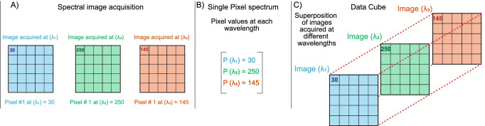
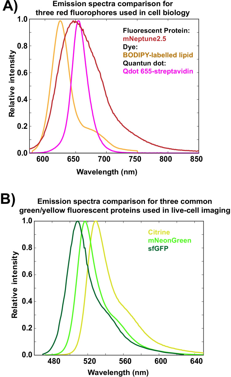
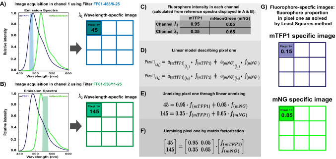
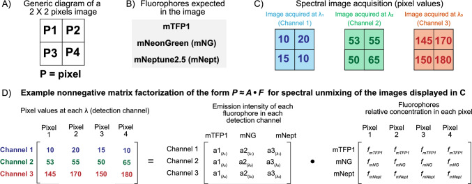
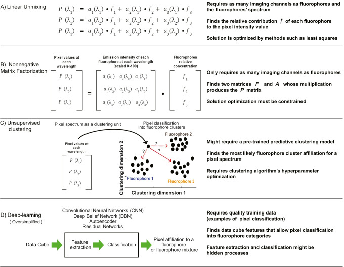
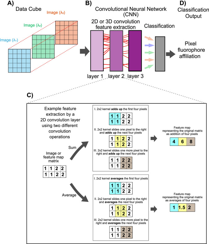
Live-cell fluorescence spectral imaging is an evolving modality of microscopy that uses specific properties of fluorophores, such as excitation or emission spectra, to detect multiple molecules and structures in intact cells. The main challenge of analyzing live-cell fluorescence spectral imaging data is the precise quantification of fluorescent molecules despite the weak signals and high noise found when imaging living cells under non-phototoxic conditions. Beyond the optimization of fluorophores and microscopy setups, quantifying multiple fluorophores requires algorithms that separate or unmix the contributions of the numerous fluorescent signals recorded at the single pixel level. This review aims to provide both the experimental scientist and the data analyst with a straightforward description of the evolution of spectral unmixing algorithms for fluorescence live-cell imaging. We show how the initial systems of linear equations used to determine the concentration of fluorophores in a pixel progressively evolved into matrix factorization, clustering, and deep learning approaches. We outline potential future trends on combining fluorescence spectral imaging with label-free detection methods, fluorescence lifetime imaging, and deep learning image analysis.

Keywords: Cell biology; Data science; Fluorescence; Live-cell imaging; Spectral imaging.

Fig. 1

Schematic definition of spectral imaging, pixel spectrum, and data cube. A Schematic representation of three images acquired at different $\mathit{\lambda }$ wavelengths (colors) using a spectral imaging setup. The intensity value of pixel number one is shown to ease comparison. B Representation of the single pixel spectrum as the values of pixel number one arranged as a vector. C Schematic representation of a data cube in which, besides their length and width dimensions, the images acquire a third dimension along their $\mathit{\lambda }$ values

Fig. 2

Emission spectra comparison among common fluorophores and fluorescent proteins used in cell biology. A Reference emission spectra comparison of three fluorophores with similar emission peaks used in cell biology applications: the red fluorescent protein, mNeptune2.5 (Chu et al. 2014); the red lipid-conjugated BODIPY dye, CellTrace™ BODIPY® TR methyl ester (NCBI 2021); and Invitrogen™'s streptavidin-conjugated red quantum dot, Qdot® 655. Notice mNeptune2.5’s broader spectrum. B Reference emission spectra comparison of superfolder green fluorescent protein (sfGFP) (Pédelacq et al. 2006), mNeonGreen (Shaner et al. 2013), and Citrine (Griesbeck et al. 2001), three green/yellow fluorophores commonly used as genetically encoded tags to fluorescently label proteins. Despite the differences in their emission peaks, the fluorophores’ spectra significantly overlap, potentially leading to co-detection and preventing their simultaneous use in fluorescence microscopy. Spectra obtained from SearchLight Spectra Viewer from Semrock accessed on 11/29/2021

Fig. 3

Linear unmixing model for spectral imaging data. A–B, left Schematic image acquisition showing the reference emission spectra of monomeric teal fluorescent protein one, mTFP1 (Ai et al. 2006), and the monomeric green fluorescent protein mNeonGreen (Shaner et al. 2013). The shaded area indicates the wavelength range of the detection channel generated using the bandpass filters A FF01-488/6–25 (light blue) and B FF01-530/11–25 (light green) from Semrock. A–B, right Schematic matrix representation of the mixed images collected by the wavelength-specific channels. For simplicity, only the intensity value of pixel one is shown. C Normalized fluorophores’ expected intensities at each detection channel are derived by calculating the approximated fluorophore spectrum area that falls in the wavelength range allowed by the filter set (shaded areas in A). D Linear model showing the intensity value of pixel number one as a linear combination of the multiplication of each fluorophore's expected intensity $\mathit{a}$ by each fluorophore’s relative concentration $\mathit{f}$ at the imaging wavelength range $\mathit{\lambda }$. E Linear equation system to solve the relative concentration of fluorophores $\mathit{f}$ in pixel number one. F Matrix factorization representation of the linear equation system to solve the relative concentration of fluorophores $\mathit{f}$ in pixel number one. G Schematic unmixed fluorophore-specific images showing the linear unmixing solution of pixel number one as approximated by the least squares method (Lloyd 1982a) using the Python function numpy.linalg.lstsq()

Fig. 4

Schematic nonnegative matrix factorization spectral unmixing. A Generic diagram of a 2 × 2 pixels image. B Fluorophores assumed to be present in the image. C Spectral image acquisition using three different detection channels showing individual pixel values. D Example of a nonnegative matrix factorization algorithm that could calculate the relative fluorophore concentration in each pixel. Notice how, in this approach, each 2 × 2 image is “unraveled” into a 1 × 4 row vector whose concatenation creates the matrix to be factorized

Fig. 5

Evolution of spectral unmixing models. A System of linear equations to solve the relative concentration of three fluorophores in a mixed pixel $\mathit{p}$. The pixel intensity value is assumed to be the sum of terms composed of each fluorophore’s expected intensity $\mathit{a}$ multiplied by each fluorophore’s relative concentration $\mathit{f}$ at the imaging wavelength $\mathit{\lambda }$. B Matrix factorization representation of a linear equation system to solve the relative concentration of fluorophores in a pixel. The pixel values matrix $\mathit{P}$ is assumed to result from multiplying the fluorophore expected intensities matrix $\mathit{A}$ by the fluorophore relative concentrations matrix $\mathit{F}$. C A clustering approach for assigning a single pixel spectrum to a particular fluorophore that is represented as a data cluster. Notice how the single pixel spectrum could be compressed to a single value in the clustering space (solid arrow) before being affiliated to a cluster by calculating, for instance, the minimum Euclidean distance between the pixel spectrum data point and the center (centroid) of the clusters representing different fluorophores (red dotted arrows). D Deep learning approach to spectral unmixing. Instead of assuming linearity or focusing on the single pixel spectrum, deep learning approaches use the entire data cube to find relevant features or patterns for single pixel classification into fluorophores. Green arrows represent an oversimplified information flow in a deep learning architecture designed to extract features (feature extraction) from a data cube and classify pixels (classification) according to fluorophores

Fig. 6

Schematic representation of a convolutional neural network (CNN) for data cube analysis using 2D convolution. A A data cube, or any other multidimensional representation of the spectral imaging data, is used as input for deep learning approaches. B The schematic CNN uses three feature extraction layers to produce feature maps of the data cube. The feature extraction process through convolution is continued in each layer using the feature maps produced by the previous layer as input. C Minimalistic schematic of feature extraction through convolution in which a kernel, or defined area in pixels, is used to scan a feature map image using two different oversimplified operations, “sum” and “average.” Notice how the original feature map image has two rows and four columns, whereas, after convolution, it is reduced to one row of three pixels containing the result of the scanning process. The deep learning algorithms can find pixel classification-relevant features by selecting the feature maps that lead to successful pixel classification based on training data. D Based on features found to be good predictors of a pixel’s fluorophore affiliation, pixels in the data cube are assigned to fluorophores or combinations of fluorophores

References

-
- Abdeladim L, Matho KS, Clavreul S, Mahou P, Sintes JM, Solinas X, Arganda-Carreras I, Turney SG, Lichtman JW, Chessel A, Bemelmans AP, Loulier K, Supatto W, Livet J, Beaurepaire E. Multicolor multiscale brain imaging with chromatic multiphoton serial microscopy. Nat Commun. 2019;10:1662. doi: 10.1038/s41467-019-09552-9. - DOI - PMC - PubMed
- Aggarwal HK, Majumdar A. Hyperspectral unmixing in the presence of mixed noise using joint-sparsity and total variation. IEEE Journal of Selected Topics in Applied Earth Observations and Remote Sensing. 2016;9:4257–4266. doi: 10.1109/JSTARS.2016.2521898. - DOI
Publication types
Grants and funding
LinkOut - more resources
Full Text Sources