GraFT: Graph Filtered Temporal Dictionary Learning for Functional Neural Imaging

Abstract

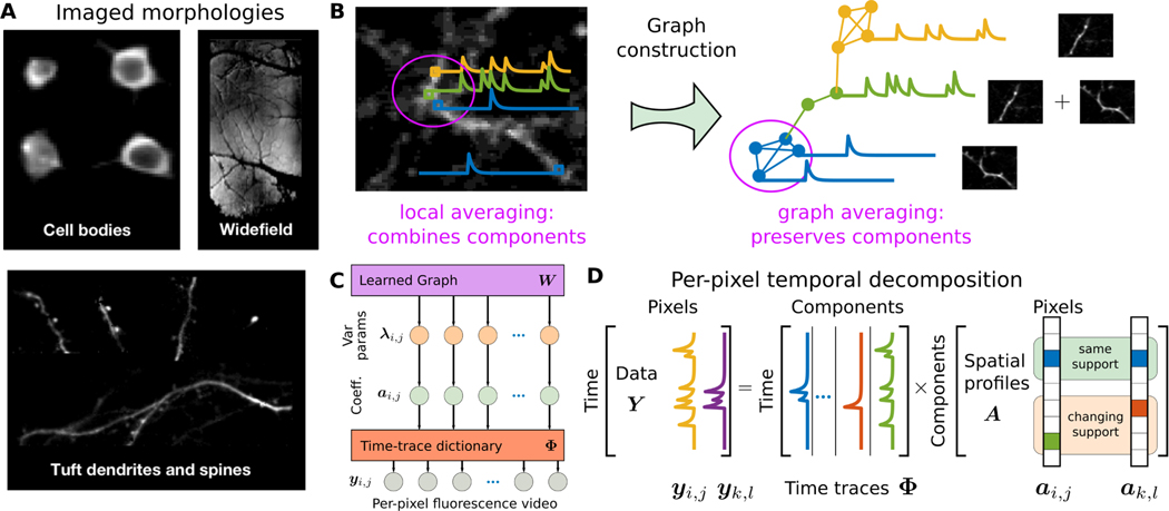
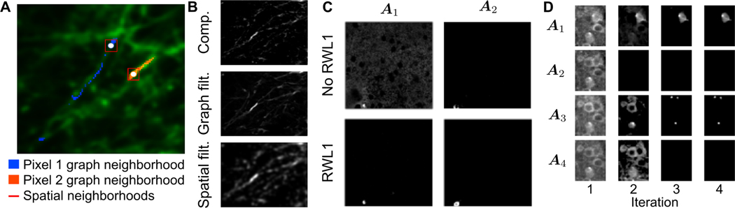
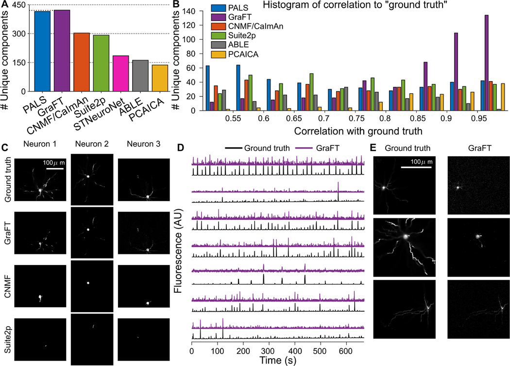
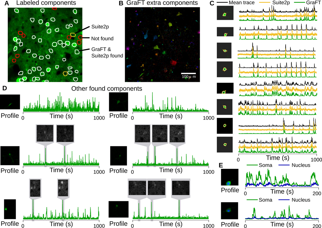
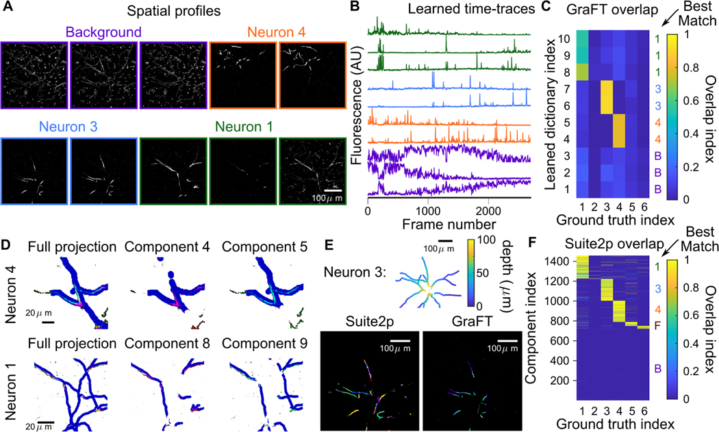
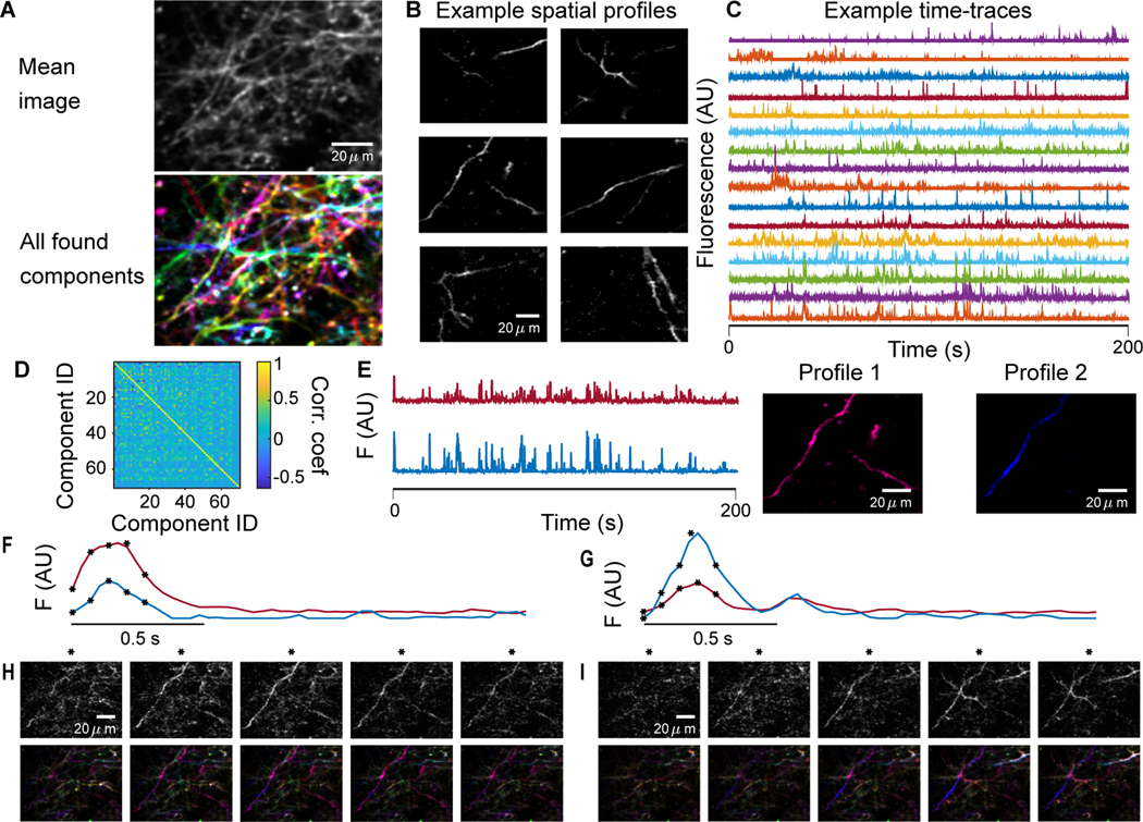
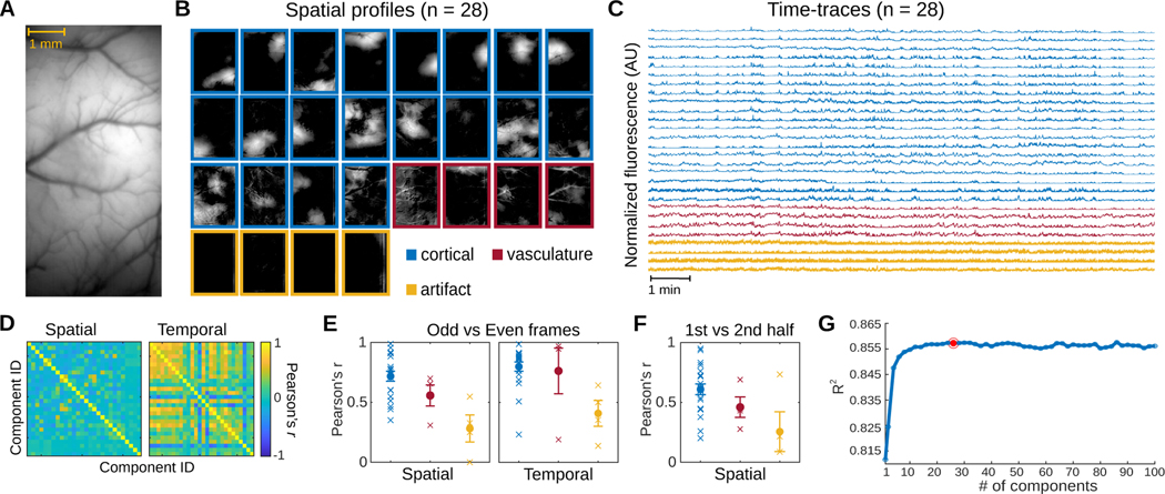
Optical imaging of calcium signals in the brain has enabled researchers to observe the activity of hundreds-to-thousands of individual neurons simultaneously. Current methods predominantly use morphological information, typically focusing on expected shapes of cell bodies, to better identify neurons in the field-of-view. The explicit shape constraints limit the applicability of automated cell identification to other important imaging scales with more complex morphologies, e.g., dendritic or widefield imaging. Specifically, fluorescing components may be broken up, incompletely found, or merged in ways that do not accurately describe the underlying neural activity. Here we present Graph Filtered Temporal Dictionary (GraFT), a new approach that frames the problem of isolating independent fluorescing components as a dictionary learning problem. Specifically, we focus on the time-traces-the main quantity used in scientific discovery-and learn a time trace dictionary with the spatial maps acting as the presence coefficients encoding which pixels the time-traces are active in. Furthermore, we present a novel graph filtering model which redefines connectivity between pixels in terms of their shared temporal activity, rather than spatial proximity. This model greatly eases the ability of our method to handle data with complex non-local spatial structure. We demonstrate important properties of our method, such as robustness to morphology, simultaneously detecting different neuronal types, and implicitly inferring number of neurons, on both synthetic data and real data examples. Specifically, we demonstrate applications of our method to calcium imaging both at the dendritic, somatic, and widefield scales.

Fig. 1.

Graph-based dictionary learning for calcium image analysis. A: Optical imaging of different neural components at different scales. B: In calcium imaging, distant pixels might be highly correlated while neighboring pixels might be very different. For example, for two crossing dendrites any technique based on local averaging is prone to corruption by competing signals. By reorganizing the pixel relationships into a data-drive graph, local averaging defined by the graph can make more judicious use of temporal correlations between pixels and extract better signal estimates. C: The graphical model of GraFT organizes variables into three layers: a set of variance parameters interconnected by the data-driven graph W, a set of sparse coefficients conditioned on the parameters, and the observed fluorescence video which is linearly generated by the coefficients through the dictionary Φ. D: Matrix factorization model: GraFT emphasizes the role of time-traces and decomposes the data into a dictionary of component time-traces and correspoding spatial maps.

Fig. 2.

GraFT regularization effects. A. Mean projection of dense dendritic imaging. The graph neighborhood of two pixels (white points)—overlaid in blue and orange—respect the geometry of the underlying dendrites and extend far along them, compared to the extent of a spatial neighborhood of 7 × 7 (red squares). B. Graph filtering applied to estimated sparse components is limited to the pixels along dendritic structures, whereas spatial filtering blurs the pixels, incorporating information from the background into the inference. C. The RWL1 filtering becomes important for suppressing background activity (left) and finding all pixels within a component (right). D. Frobenius norm in the DL cost enables components “turning off”, thus leading to more accurate learning of the number of components in the data.

Fig. 3.

Assessment of GraFT and competing methods on anatomically-based calcium imaging simulations. A: The number of unique neurons found with each method. B: Histogram of temporal correlations between extracted time-traces and the ground truth traces. The GraFT dictionary better matches the ground-truth compared to other methods. C: GraFT finds more complete spatial profiles for neurons that are also identified by other methods, and dendrites are better identified. D: Time-traces for neurons not found via other methods correlate well with ground truth traces, but have low SNR. E: Neurons found only with GraFT tend to have less localized spatial profiles.

Fig. 4.

Somatic imaging from NeuroFinder. A: Mean projection of the field-of-view (green) with overlay of all manually identified cells. Most cells are identified by both GraFT and Suite2p (white), some (red) were not identified at all (i.e., due to inactivity), and a couple were identified only by Suite2p (yellow). B: All non-background (well-isolated) profiles found by GraFT that were not in the ground-truth, including many apical dendrites, several somatic components and other small components. C: Comparison of the average trace of the manually labeled spatial profile with GraFT and Suite2p time-traces. D: Additional identified components beyond the manual labels exhibited smaller, dendritic structure, even when these are in proximity to brighter somatic components (right column, middle). Local averages of frames from the movie demonstrate that these components do exist in the data and were simply not labeled manually. E: The sensitivity of GraFT enables for the cytoplasmic (green) and nuclear (blue) portions of individual neurons to be identified.

Fig. 5.

Sparse dendrite data. A-B: 10 temporal dictionary elements and 10 corresponding spatial maps identified with GraFT. Dendritic components extend throughout the entire image. C: Correlations of GraFT components with anatomical labels. D: The two identified components found per ground truth structure (colored in red and green channels) overlap with slightly different portions of the dendritic structure (dilated in blue). The full ground truth projected onto one image on the right column, and the middle and right plots showing the ground truth at slices shifted by 2 μm. This reveals that each component corresponds to a slightly different axial portion of the neuron, indicating that the difference is due to axial motion. E: Suite2p run in “dendrite” mode identifies approximately 200 ROIs for Neuron 3 (different colors in the lower-left plot) comprise this single neuron. GraFT picks up the same neuron with two components: each corresponding to a different depth. F: Correlations of Suite2p ROIs with anatomical labels.

Fig. 6.

Dense dendrite data. A: Many fluorescing components are highly overlapping as seen in the mean projection (top). GraFT identifies 60 components in this dataset (bottom; each component is plotted with a different color). B: Examples of spatial maps recovered by GraFT. C: Example time-traces demonstrate a diversity of activity patterns that overlap in time. D: Correlation matrix of the estimated time-traces indicates the decomposition is capturing sufficiently different time-traces. E: The two highest correlated time-traces, along with the corresponding spatial maps, indicate these two overlap significantly, perhaps both representing pieces of one true dendritic component. F-I: Closer inspection of the spatial profiles reveals that profile 2 actually represents a different process in the dendrite centered around a spine in the lower-left-hand corner of the image. Two example bursts of activity (F and G) demonstrate that these components have different activity at different times. Frames from the starred time-points in F and G are shown in H and I respectively, with the raw data frame in the top row and the reconstruction in the bottom row.

Fig. 7.

Widefield data. A. The imaged cross-cortical field-of-view. B. GraFT spatial maps when run with n = 28 components. Three main classes of components can be identified: broad cortical activity (blue), vasculature-based fluorescence (red), and imaging artifacts (yellow). C. Time-traces for the n = 28 case, color coded by the class of the component. D. GraFT demonstrates inference consistency, as demonstrated by comparing the learned time-traces and spatial maps for GraFT run only on the odd and even frames separately. Pearson’s correlation between best-matched spatial and temporal maps are very high for all maps and dictionary elements for the case of n = 28. E. Breakdown of the diagonal elements of the correlation matrix in D by class (cortical, vascular, and artifactual). The learned spatial maps and time-traces for cortical maps was the most consistent, with the highest correlation values. F. A similar analysis of spatial maps learned separately across the first half and the second half of the imaging session for n = 28 demonstrates that consistent cortical areas are observed during the same behavior even over different epochs. G. Variance explained as a function of the number of dictionary elements shows a plateau at approximately 0.855 with ≈ 20 components.

References

1. Denk W, Strickler JH, and Webb WW, “Two-photon laser scanning fluorescence microscopy,” Science, vol. 248, no. 4951, pp. 73–6, 1990. [Online]. Available: http://www.ncbi.nlm.nih.gov/pubmed/2321027 - PubMed
1. Mank M. and Griesbeck O, “Genetically encoded calcium indicators,” Chem Rev, vol. 108, no. 5, pp. 1550–64, 2008. [Online]. Available: http://www.ncbi.nlm.nih.gov/pubmed/18447377 - PubMed
1. Tian L, Akerboom J, Schreiter ER, and Looger LL, “Neural activity imaging with genetically encoded calcium indicators,” Prog Brain Res, vol. 196, pp. 79–94, 2012. [Online]. Available: http://www.ncbi.nlm.nih.gov/pubmed/22341322 - PubMed
1. Jung JC, Mehta AD, Aksay E, Stepnoski R, and Schnitzer MJ, “In vivo mammalian brain imaging using one-and two-photon fluorescence microendoscopy,” Journal of neurophysiology, vol. 92, no. 5, pp. 3121–3133, 2004. - PMC - PubMed
1. Rodriguez C, Liang Y, Lu R, and Ji N, “Three-photon fluorescence microscopy with an axially elongated bessel focus,” Optics letters, vol. 43, no. 8, pp. 1914–1917, 2018. - PMC - PubMed