Navigable Space and Traversable Edges Differentially Influence Reorientation in Sighted and Blind Mice

Abstract

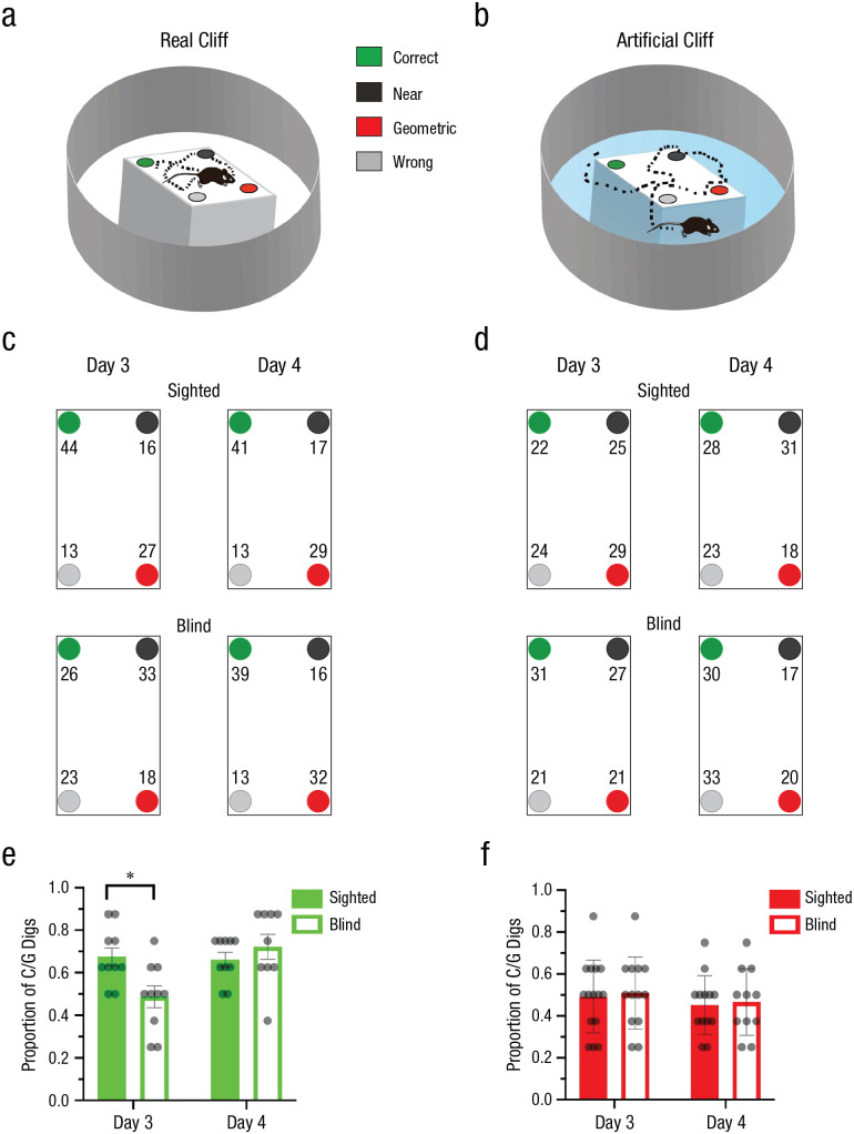
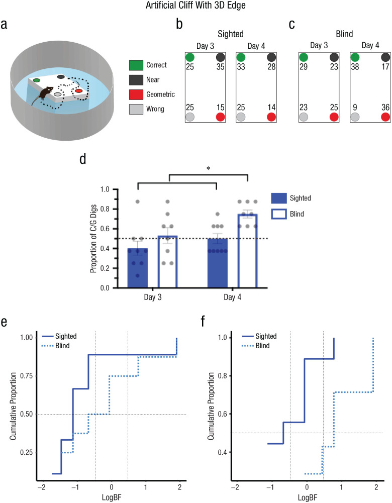
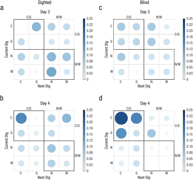
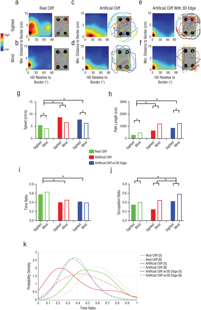
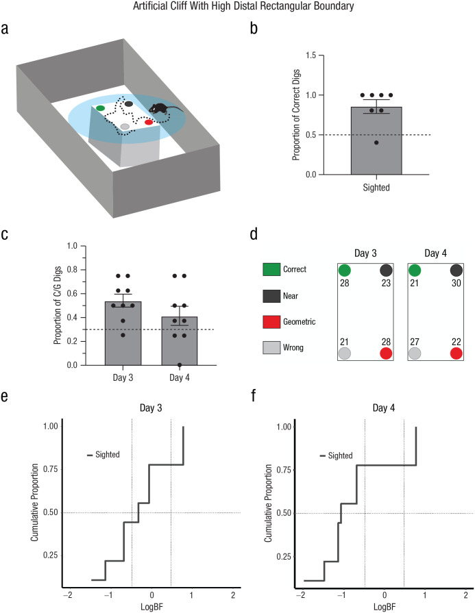
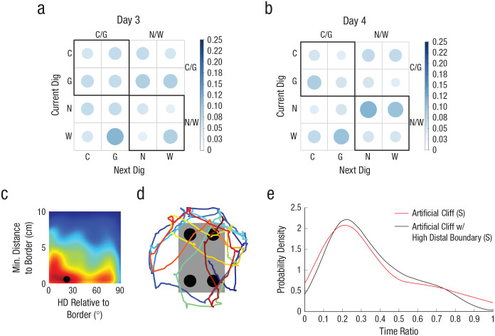
Reorientation enables navigators to regain their bearings after becoming lost. Disoriented individuals primarily reorient themselves using the geometry of a layout, even when other informative cues, such as landmarks, are present. Yet the specific strategies that animals use to determine geometry are unclear. Moreover, because vision allows subjects to rapidly form precise representations of objects and background, it is unknown whether it has a deterministic role in the use of geometry. In this study, we tested sighted and congenitally blind mice (Ns = 8-11) in various settings in which global shape parameters were manipulated. Results indicated that the navigational affordances of the context-the traversable space-promote sampling of boundaries, which determines the effective use of geometric strategies in both sighted and blind mice. However, blind animals can also effectively reorient themselves using 3D edges by extensively patrolling the borders, even when the traversable space is not limited by these boundaries.

Keywords: blindness; geometric strategy; reorientation; spatial learning; spatial navigation.

Fig. 1.

Experiment 2: reorientation in the real-cliff and artificial-cliff conditions. The schematics show the experimental setup in the real-cliff (a) and artificial-cliff (b) conditions. In the real-cliff condition, animals were forced to navigate a rectangular shape, whereas in the artificial cliff, a rectangular texture was placed on a circular platform that did not limit the traversable space to the task-relevant area (i.e., the rectangle containing the four cups). The task consisted in finding a reward hidden in one of the four cups at the edges of the rectangular shape that enclosed the cup locations. In the schematics, green indicates the correct rewarded location, black indicates the location nearest to the reward along the same short wall as the reward location, red indicates the geometrically opposite corner from the reward location, and gray indicates the location not associated with the correct geometric axis or the short wall near the reward. The percentage of digs in the four different cup locations is shown for the real-cliff (c) and artificial-cliff (d) conditions on Days 3 and 4; means are shown for sighted mice in the upper row and blind mice in the lower row. Results are shown separately for each cup location, using the color codes shown in (a) and (b). Digging preference (proportion of first digs in the geometrically correct axis relative to the total number of digs) is shown for sighted and blind mice in the real-cliff (e) and artificial-cliff (f) conditions on Days 3 and 4. Bars show means (error bars indicate standard errors of the mean), and dots represent individual data. The asterisk indicates a significant difference between means for sighted and blind mice (α = .05). Real-cliff condition: sighted mice: n = 10, blind mice: n = 9; artificial-cliff condition: sighted mice: n = 12, blind mice: n = 11.

Fig. 2.

Experiment 2: results of the hierarchical Bayesian analysis at the individual and group levels. The cumulative proportion of subjects in terms of the weight of evidence is shown for the real-cliff condition on Day 3 (a) and Day 4 (b) and the artificial-cliff condition on Day 3 (c) and Day 4 (d). Conventional values showing the border marking credibility for the null hypothesis (chance performance) and the alternative hypothesis (use of geometry) are indicated by vertical dashed lines, log(1/3) = −0.48 and log(3) = 0.48. The value of half (0.5) of the sample is marked by a horizontal dashed line. LogBFs > 0.48 indicate credibility for the alternative hypothesis (geometric learning), whereas logBFs < –0.48 indicate credibility for the null hypothesis (chance performance).

Fig. 3.

Experiment 2: results of the probability analysis of digging sequence in the real-cliff (a–d) and artificial-cliff (e–h) conditions, separately for sighted mice (left column) and blind mice (right column) on Day 3 and Day 4 (upper and lower rows, respectively, for each group of subjects). The bar on the right of each graph indicates probability. Larger, darker circles indicate higher probability; smaller, lighter circles indicate lower probability. C = correct corner; G = geometrically equivalent corner; N = near location to rewarded cup; W = wrong location.

Fig. 4.

Experiment 3: reorientation in the artificial-cliff-with-3D-edge condition. A schematic of the arena is shown in (a). The environment was identical to the artificial cliff, but the rectangular shape in the center of the arena was elevated, creating a 3D edge that did not limit the traversable space. The task consisted in finding a reward hidden in one of four cups at the edges of the elevated rectangular shape that enclosed the cup locations. In the schematic, green indicates the correct rewarded location, black indicates the location nearest to the reward along the same short wall as the reward location, red indicates the geometrically opposite corner from the reward location, and gray indicates the location not associated with the correct geometric axis or the short wall near the reward. The percentage of digs in the four different cup locations is shown for sighted (b) and blind (c) mice on Days 3 and 4. Results are shown separately for each cup location, using the color codes shown in (a) and (b). Digging preference (proportion of first digs in the geometrically correct axis relative to the total number of digs) is shown (d) for sighted and blind mice on Day 4. Bars show means (error bars indicate standard errors of the mean), and dots represent individual data. The asterisks indicates significant differences between group performance on different days (α = .05). The cumulative proportion of subjects in terms of the weight of evidence supporting either the null hypothesis (H_null; chance performance) or the alternative hypothesis (H_alt; use of geometry) is shown for sighted and blind mice on Day 3 (e) and Day 4 (f). Conventional values showing the border marking credibility for H_null versus H_alt are indicated by vertical dashed lines, log(1/3) = −0.48 and log(3) = 0.48. The value of half (0.5) of the sample is marked by a horizontal dashed line. Sighted mice: n = 9, blind mice: n = 8.

Fig. 5.

Experiment 3: results of the probability analysis of digging sequence in the artificial-cliff-with-3D-edge condition, separately for sighted mice (a, b) and blind mice (c, d) on Day 3 and Day 4 (upper and lower rows, respectively, for each group of subjects). The bar on the right of each graph indicates probability. Larger, darker circles indicate higher probability; smaller, lighter circles indicate lower probability. C = correct corner; G = geometrically equivalent corner; N = near location to rewarded cup; W = wrong location.

Fig. 6.

Experiment 3: results of the path analysis. Distance and heading orientation relative to border and sample paths from Day 4 in the real cliff (a, b), artificial cliff (c, d), and artificial-cliff-with-3D-edge (e, f) conditions is shown for sighted and blind mice (upper and lower row, respectively). The relative heading direction (HD) and distance to the task-relevant border (rectangle) were calculated for each path segment and added to the associated bin. Average color-coded maps show the heading orientation (x-axis) and distance from border (y-axis) distributions. Along the x-axis indicates, 0° indicates parallel and 90° indicates perpendicular heading to the border. The black dot indicates the location of the maximum orientation/distance. In all path diagrams, blue indicates the beginning of the path, and dark red indicates the first dig location. Speed and path length are shown in (g) and (h), respectively, for sighted and blind mice in each of the three conditions. Time and occupancy ratio are shown in (i) and (j), respectively, for sighted and blind mice in each of the three conditions. In (g–j), bars show means (error bars indicate standard errors of the mean), and dots represent individual data. The asterisks indicates significant differences between groups or between group performance on different days (α = .05). The density distribution of time ratios (k) shows the amount of time sighted and blind mice spent at the border in each condition. S = sighted; B = blind.

Fig. 7.

Experiment 4: reorientation in the artificial-cliff-with-high-distal-rectangular-boundary condition. A schematic of the arena is shown in (a). The context was identical to the artificial cliff but was surrounded by a large rectangular shape. The task consisted in finding a reward hidden in one of four cups at the edges of the rectangular shape that enclosed the cup locations, which was placed on a circular platform. In the schematic, green indicates the correct rewarded location, black indicates the location nearest to the reward along the same short wall as the reward location, red indicates the geometrically opposite corner from the reward location, and gray indicates the location not associated with the correct geometric axis or the short wall near the reward. The proportion of correct digs (b) is shown for sighted mice. Digging preference (proportion of first digs in the geometrically correct axis relative to the total number of digs) is shown in (c) for Days 3 and 4. Bars show means (error bars indicate standard errors of the mean), and dots represent individual data. The dashed line indicates chance performance. The percentage of digs in the four different cup locations is shown (d) for Days 3 and 4. Results are shown separately for each cup location, using the color codes shown in (a) and (b). The cumulative proportion of subjects in terms of the weight of evidence supporting either the null hypothesis (H_null; chance performance) or the alternative hypothesis (H_alt; use of geometry) is shown for Day 3 (e) and Day 4 (f). Conventional values showing the border marking credibility for H_null versus H_alt are indicated by vertical dashed lines, log(1/3) = −0.48 and log(3) = 0.48. The value of half (0.5) of the sample is marked by a horizontal dashed line.

Fig. 8.

Experiment 4: results of the sequential digging probability and path analysis in the artificial-cliff-with-high-distal-rectangular-boundary condition in sighted mice. Sequential digging probability is shown for Day 3 (a) and Day 4 (b). The bar on the right of each graph indicates probability. Larger, darker circles indicate higher probability; smaller, lighter circles indicate lower probability. C = correct corner; G = geometrically equivalent corner; N = near location to rewarded cup; W = wrong location. The average heading direction (HD) relative to the border is shown in (c). Along the x-axis indicates, 0° indicates parallel and 90° indicates perpendicular heading to the border. The black dot indicates the location of the highest value for head direction and distance to border. A sample path illustrating border crossings rather than parallel patrolling is shown in (d). The time-ratio density distribution (e) shows the amount of time sighted mice spent at the border in each condition. Sighted (S) mice: n = 9.

References

1. Alexander A. S., Carstensen L. C., Hinman J. R., Raudies F., Chapman G. W., Hasselmo M. E. (2020). Egocentric boundary vector tuning of the retrosplenial cortex. Science Advances, 6(8), Article eaaz2322. 10.1126/sciadv.aaz2322 - DOI - PMC - PubMed
1. Anderson M. I., Jeffery K. J. (2003). Heterogeneous modulation of place cell firing by changes in context. The Journal of Neuroscience, 23(26), 8827–8835. - PMC - PubMed
1. Aronov D., Nevers R., Tank D. W. (2017). Mapping of a non-spatial dimension by the hippocampal-entorhinal circuit. Nature, 543(7647), 719–722. - PMC - PubMed
1. Bleckmann H., Zelick R. (2009). Lateral line system of fish. Integrative Zoology, 4(1), 13–25. - PubMed
1. Bonner M. F., Epstein R. A. (2017). Coding of navigational affordances in the human visual system. Proceedings of the National Academy of Sciences, USA, 114(18), 4793–4798. - PMC - PubMed
Publication types
LinkOut - more resources