1H-Detected Biomolecular NMR under Fast Magic-Angle Spinning

Abstract

Since the first pioneering studies on small deuterated peptides dating more than 20 years ago, ¹H detection has evolved into the most efficient approach for investigation of biomolecular structure, dynamics, and interactions by solid-state NMR. The development of faster and faster magic-angle spinning (MAS) rates (up to 150 kHz today) at ultrahigh magnetic fields has triggered a real revolution in the field. This new spinning regime reduces the ¹H-¹H dipolar couplings, so that a direct detection of ¹H signals, for long impossible without proton dilution, has become possible at high resolution. The switch from the traditional MAS NMR approaches with ¹³C and ¹⁵N detection to ¹H boosts the signal by more than an order of magnitude, accelerating the site-specific analysis and opening the way to more complex immobilized biological systems of higher molecular weight and available in limited amounts. This paper reviews the concepts underlying this recent leap forward in sensitivity and resolution, presents a detailed description of the experimental aspects of acquisition of multidimensional correlation spectra with fast MAS, and summarizes the most successful strategies for the assignment of the resonances and for the elucidation of protein structure and conformational dynamics. It finally outlines the many examples where ¹H-detected MAS NMR has contributed to the detailed characterization of a variety of crystalline and noncrystalline biomolecular targets involved in biological processes ranging from catalysis through drug binding, viral infectivity, amyloid fibril formation, to transport across lipid membranes.

Figure 1

Schematic showing the different sources of spectral line broadening in solid-state MAS NMR and how they contribute to the final lineshape. Both the incoherent and coherent homogeneous broadening is assumed to be Lorentzian, and all sources of inhomogeneous broadening are assumed to be Gaussian.

Figure 2

Homogeneous incoherent contribution to ¹H linewidths (¹H Δ^inc) calculated with eq 3, with a homonuclear coupling to a proton at a distance of 3 Å, heteronuclear coupling with the bonded ¹⁵N at a distance of 1.04 Å, and 10 ppm of ¹H CSA. The correlation functions were calculated with the simple model-free approach, with S² set to 0.9 and τ_c varied between 10^–8 and 10^–3 s. One should note that the values given here are only semiquantitative as Redfield theory is not a rigorous approach for the slowest motions (largest τ_c).

Figure 3

Experimental ¹³C and ¹H solid-state MAS NMR spectra of natural abundance glycine acquired at increasing spinning frequencies. The ¹³C spectra shown in (a) were acquired under broadband heteronuclear ¹H decoupling, and so the coherent homogeneous contribution to the linewidth of the spinning side-bands is largely suppressed, and the total linewidth is largely independent of MAS frequency. By contrast, the ¹H spectra in (b) were not acquired with any decoupling sequence, and so the coherent homogeneous linewidth is dominant and decreases with increasing MAS frequency.

Figure 4

2D amide ¹H–¹⁵N (a–d) and methyl ¹H–¹³C (f–h) correlation spectra acquired at variable MAS frequencies [(a) 20, (b,f) 40, (c,g) 60, and (d,h) 111 kHz] on a microcrystalline sample of protonated GB1 (structure displayed with hydrogen atoms in blue in panel e).

Figure 5

(a) Bulk T′₂ of amide (black) and methyl ¹H (gray) in a microcrystalline sample of nondeuterated GB1 plotted versus MAS frequency (at field strength B₀ = 23.5 T). (b−c) Total linewidths, Δ^tot, of amide (black) and methyl ¹H (gray) of residue T11 as a function of the MAS frequency (ν_r linear with the x-axis in b, and τ_r linear with the x-axis in c). T′₂ values translate into homogeneous contributions, Δ^hom, and for amide ¹H of residue T11 are depicted in (c) along with total linewidths, Δ^tot, and the fitted inhomogeneous contribution, Δ^inhom.

Figure 6

2D ¹H–¹⁵N (top) and ¹H–¹³C (bottom) correlation spectra acquired at 100 kHz MAS frequency for (a) microcrystalline maltose binding protein, (b) tubular HIV-1 capsid protein assemblies, (c) 26mer box C/D RNA bound to the L7Ae protein, (d) membrane protein AlkL, and (e) fibrils of Aβ₄₂. Displayed regions correspond to amide and α sites (a,b,d,e) and imino N–H and ribose C1′–H1′ and U/C C5–H5 moieties (c). The corresponding structures (PDB codes 1ANF, 6WAP, 2N0R, 6QWR, 5KK3) are displayed on top of each pair of spectra.

Figure 7

Sensitivity gains by detecting on ¹H with respect to heteronuclei (X being ¹⁵N or ¹³C). Virtual RF irradiation schemes for measuring 2D ¹H–X correlations with (a) heteronuclei detection and (b) proton detection. Excitation pulses are depicted as black rectangles; indirect chemical shift encoding is performed during the t₁ evolution time, and transfer sequences are shown as orange blocks. (c) Sensitivity gain factors ξ are calculated with eq 12 with linewidths (W) measured on a fully protonated microcrystalline GB1 sample: W_H = 220, 156, 120, 102, 95 Hz (at 40, 60, 80, 100, 111 kHz MAS, respectively), W_C = 105 Hz, and W_N = 55 Hz. Both W_C and W_N are supposed to be constant over the 20–111 kHz MAS frequency range.

Figure 8

Comparison of six Bruker rotors spinning at MAS frequencies up to 111 kHz. The rotor outer diameters are indicated, while a pencil serves as a scale reference.

Figure 9

Detection sensitivity as the function of MAS frequency (thus also rotor size) for ¹³C and ¹H nuclei. (a) Rotor inner volume for different commercial rotors (Bruker 3.2, 2.5, 1.3, and 0.7 mm) is depicted an orange area. The detection sensitivity of the probe, calculated as the product of the sample volume and the inverse of the rotor diameter, is shown in blue in the same plot. Values are normalized to the detection sensitivity of a Bruker 3.2 mm probe. (b) Mass sensitivity of a direct proton 1D experiment (yellow) as compared to ¹³C-detected 1D CP (purple) versus MAS. CP efficiency of 50% was assumed. Increasing MAS reduces homogeneous contribution to ¹H linewidths, which in turn translates into better sensitivity. Simulations are performed for different inhomogeneous contributions to the lines (from 0 to 200 Hz, dashed lines) and calculated values for microcrystalline GB1 correspond to the solid line (60 Hz inhomogeneous linewidth). ¹³C LW are supposed to be identical in the whole MAS range, corresponding to constant mass sensitivity. Values are normalized to ¹H detection at 111 kHz MAS (with Δ^inhom = 60 Hz). (c) Product of the probe detection sensitivity and the mass sensitivity is given as the absolute sensitivity of ¹H detection (yellow) and ¹³C detection (purple). Values are normalized to ¹³C detection at 20 kHz MAS.

Figure 10

Proton dilution for high-resolution proton detection. The general dilution scheme is shown in (a) for an arbitrary spin network. In (b), the protons of SH3 are depicted for full protonation, exchangeable protons only, and finally, 10% exchangeable protons at random. 2D ¹H–¹⁵N correlation spectra of a perdeuterated sample of microcrystalline SH3 with (c) 100% back-exchange and (d) 10% back-exchange acquired at 13 kHz MAS frequency at a magnetic field of 14.1 T. Reproduced with permission from ref (85) (copyright 2006 John Wiley & Sons) and ref (3) (copyright 2012 Elsevier).

Figure 11

(a) Evolution of the mass sensitivity of ¹H-detected experiments with MAS rates, estimated for different labeling schemes: ¹H (100%) natural abundance (yellow), perdeuteration with 10% (light blue), 30% (medium blue), and 100% (dark blue) proton back-exchange at labile sites. ¹H sensitivity is assumed to be proportional to αW_H^–1/2, where α is the level of protonation at the labile sites and W_H is the ¹H linewidth. The latter parameter is as measured on GB1 (for 100% ¹H^N and 100% ¹H) or calculated with an inhomogeneous contribution of 60 Hz and homogeneous contributions extrapolated from refs (86) (for 10% ¹H^N) and (87) (for 30% ¹H^N). Similarly to Figure 8b, mass sensitivity is given with respect to 100% ¹H samples spun at 111 kHz. (b) Absolute sensitivity of ¹H-detected experiments, calculated as the product of probe detection sensitivity from Figure 8a and mass sensitivity. Values are indicated for the four labeling schemes of panel a with the same color code. Arrows indicate the conditions that maximize sensitivity without compromising resolution for each sample preparation. As in Figure 8c, the reference sensitivity is that of ¹³C detection in a Bruker 3.2 mm rotor at 20 kHz MAS.

Figure 12

Schematic representation of labeling schemes in a valine–alanine fragment. The nuclei present in natural abundance (C, N, O) and deuterons are colored in gray, ¹³C in black, and ¹H in red. For positions that are only partially labeled in the protein, the rough ¹H/²D ratio is indicated by a red/gray pie chart.

Figure 13

Homogeneous linewidths reported in the literature for protonated (black) and perdeuterated samples with 100% back-exchange of labile protons (red), at 23.5 T B₀ field: GB1, microcrystalline β1 immunoglobulin binding domain of protein G (triangles); SOD, microcrystalline Cu^I,Zn^II-loaded dimeric superoxide dismutase (ellipses); AP205, Acinetobacter phage 205 coat protein (stars); AlkL, outer-membrane alkane transporter from Pseudomonas putida (hexagons); and at 20.0 T B₀ field strength: UBQ, microcrystalline human ubiquitin (squares and filled circles); CP149, hepatitis B viral capsid core protein (open circles). For ubiquitin, three sets of experimental values correspond to the studies by Penzel et al. (squares), Penzel et al. (filled circles), and Schleedorn et al. and dashed lines to the fits reported therein (valid for B₀ ≈ 20.0 T). The right panel shows a close-up view for MAS rates above 100 kHz, indicating the putative MAS rate (ν_r ≃500 kHz) for which protonated samples will reach the coherent linewidth (red horizontal line) of deuterated samples spun at 100 kHz. Similarly, the gray horizontal line indicates a hypothetical MAS rate required for a protonated (ν_r ≃ 1200 kHz) and a deuterated (ν_r ≃350 kHz) sample to match ¹H resolution observed in solution NMR for a small protein of MW = 10 kDa (τ_c ≃10 ns). Note that the x-axis is linear with rotor period.

Figure 14

¹H resolution as a function of degree of sample or structural inhomogeneity (Δ^inhom). Total effective linewidth, Δ^tot (solid curves), is simulated for a range of MAS frequencies using eq 11, assuming the inhomogeneous contribution of 0.2, 0.15, 0.10, and 0.05 ppm (black, red, green, and blue solid and dashed curves, respectively), and the homogeneous contribution as determined experimentally for ν_r = 40–111 kHz for a representative amide ¹H of residue T11 in nondeuterated GB1 on 23.5 T (a) and 11.75 T (b) spectrometers. The x-axis is linear with rotor period. Note that despite a generally lower absolute linewidth (in Hz) on a 500 MHz ¹H spectrometer (b) for ν_r > 60 kHz, the actual resolution in ppm (second vertical axes) is inferior compared to that of a 23.5 T spectrometer (a).

Figure 15

Comparisons of 2D ¹H–¹³C correlation spectra at 100 kHz MAS and at two different external magnetic fields for fully protonated (a,b) microcrystalline GB1 (ω_0,H/(2π) = 500 MHz in black and 1000 MHz in red), (c) M2 embedded in lipid membrane (ω_0,H/(2π) = 950 MHz in blue and 1200 MHz in red), and (d) sedimented Rpo4/7 protein complex (ω_0,H/(2π) = 850 MHz in blue and 1200 MHz in red). Reproduced with permission from ref (118) (copyright 2021 MDPI) and ref (119) (copyright 2021 Springer Nature).

Figure 16

Evolution of resolution (a,b) and sensitivity (c,d) as a function of the external magnetic field, simulated for glycine protons. In addition to the homogeneous dipolar broadening, panels (b,d) include an inhomogeneous contribution of 0.05 ppm to the lines. Resolution is defined as the inverse of the full linewidth at half-maximum (FWHM) of the proton signal in parts per million and is calculated for 79.2 kHz (black), 100 kHz (red), 125 kHz (green), and 166.7 kHz (purple) MAS frequencies. Sensitivity was assumed to scale as B₀^3/2 and W_H^–1/2, where B₀ is the external magnetic field and W_H is the FWHM of the proton signal in hertz. Time saving was defined as the square of the sensitivity.

Figure 17

Top: Sample optimization of ¹⁵N-labeled AlkL in lipid bilayers of different compositions. (a) DPhPC, protein-to-lipid ratio 1:1, (b) DMPC, protein-to-lipid ratio 1:1 recorded on a 800 MHz spectrometer at 60 kHz MAS, (c) DMPC, protein-to-lipid ratio 2:1, recorded on a 1000 MHz spectrometer at 111 kHz MAS. Reproduced with permission from ref (12). Copyright 2018 Elsevier. Bottom: Spectral resolution as a function of LPR. Two-dimensional ¹H,¹⁵N correlation spectra of Gly- and Tyr-labeled NS4B reconstituted into PC/Chol liposomes at LPRs from 0.25 to 8 acquired at ω_H = 850 MHz and 80 kHz (d–g) or 90 kHz (h,i) MAS. Reproduced with permission from ref (108). Copyright 2020 John Wiley & Sons.

Figure 18

Schematic drawing of a solid-state NMR rotor filling tool for a swinging bucket ultracentrifuge rotor. The plot indicates the theoretical acceleration needed to sediment a protein (assembly) of a given molecular weight. Adapted with permission from ref (133). Copyright 2019 Elsevier.

Figure 19

Frictional heating induced by MAS rotors of different sizes in dependence of their spinning frequency. Parabolic fit curves are plotted as lines. Asterisks label the experimental datasets, determined by monitoring the chemical shift of lead chloride. Data points for the 0.7 mm probe are inferred from the ⁷⁹Br chemical shift of KBr following the procedure described in ref (135). In this experiment, the variable-temperature gas flow was set to 1200 L/h and regulated at 293 K. Adapted with permission from ref (134). Copyright 2017 Elsevier.

Figure 20

Spin-up and cool-down method to counter frictional heating with sample cooling in order to keep the sample temperature constant in a Bruker 0.7 mm rotor.

Figure 21

Spectral data and simplified pulse sequences for three methods to set the magic angle. (a) Classic ⁷⁹Br (KBr) method is shown on top, methods for angle adjustment directly on a protein sample rely either on (b) optimizing the ¹H T₂′ (middle) or (c) H–N J coupling spin–echo (bottom). In (b), the ¹H echo delay τ₁ is set close to T₂′/2, whereas in (c), the ¹⁵N echo delay τ₂ is set to exactly (2 J_NH)⁻¹ ≈ 10.87 ms to fully refocus ¹J_NH coupling.

Figure 22

(a) General block scheme of a multidimensional NMR experiment with ¹H detection. An RF scheme of 2D ¹H,¹⁵N or ¹H,¹³C correlation experiments employing either two (b) cross-polarizations (“CP-HSQC”) or (c) refocused scalar transfers (“J-HSQC”) between ¹H and heteronuclear spins (X).

Figure 23

Efficiency of an out-and-back scalar-coupling-based transfer between ¹H and ¹⁵N (¹J_NH = 93 Hz) as a function of ¹H refocused coherence lifetime T″₂ (neglecting efficiency loss of refocusing the antiphase to in-phase ¹⁵N coherences). Red, light blue, and blue circles correspond to ¹H^N bulk coherence lifetimes reported, respectively, for deuterated, inverse fractionally deuterated, and nondeuterated proteins. Labels denote the proteins, for which coherence lifetimes were reported in the following literature: UBQ, microcrystalline ubiquitin;^, GB1, microcrystalline β₁ Immunoglobulin Binding Domain of Protein G;^, SH3, microcrystalline chicken α-spectrin Src-homology 3; SOD, microcrystalline superoxide dismutase; SSB, gel-like precipitate of the tetrameric single-stranded DNA-binding protein; AP205 sedimented, Acinetobacter phage 205 coat protein;^, β2m_D76N, β2 microglobulin fibrils. The MAS frequency is indicated for each case.

Figure 24

Efficiency of ¹H to ¹⁵N cross-polarization (a–c,e,f) simulated in SIMPSON and (d) measured experimentally using the ¹H,¹⁵N CP-HSQC experiment with variable ¹H and ¹⁵N RF strengths (within available power limits) during the first CP performed for a microcrystalline sample of maltose binding protein at 111 kHz MAS on an 18.8 T spectrometer. Theoretical CP efficiency at (a) 20, (b) 62.5, and (c) 111 kHz MAS with DQ and ZQ conditions color coded in blue and red, respectively. Simulations (a–c) assumed a uniform B₁ field within an RF coil, the same sample amount and coil geometry in all cases, a contact time of 300 μs, and a spin system consisting of ¹⁵N and four ¹H spins (¹H^N, ¹Hα ¹Hβ₂, ¹Hβ₃) of a geometry and chemical shift tensors described in detail in ref (151). Time dependence of inhomogeneity (due to MAS) was not considered. (e) CP efficiency derived from (c) by taking into account the spatially dependent B₁ field distribution, modeled according to the Biot-Savart law in 10,000 sample voxels, and generated by an 8-loop RF coil with infinitely thin wire of a geometry closely corresponding to Bruker 0.7 mm coil design (courtesy of Frank Engleke, Bruker BioSpin GmbH). (f) CP efficiency assuming additionally a moderately ramped ¹H RF amplitude (varied from 0.9 to 1.0), as typically used for greater sensitivity and RF stability of the CP. All simulations included B₁-dependent: excitation, sample coupling to the RF coil, and additional spatial filtering by a second CP (from ¹⁵N to ¹H). (g,h) Simulated relative efficiency of (g) ¹H to ¹⁵N (“forward”) and (h) ¹⁵N to ¹H (“backward”) CP as a function of a contact time for the cases where the ¹H RF amplitude is either constant (blue curve) or linearly varied from 0.8, 0.7, or 0.5 to 1.0 of the maximum RF over contact time (green, magenta, and orange curves, respectively).

Figure 25

Relevance of sample hydration and efficiency of water signal suppression in ¹H-detected MAS NMR. (a) Effect of gradual sample dehydration due to improper sealing of the rotor observed in ¹H 1D spectra that lead to degradation of resolution of ¹H and ¹⁵N resonances. (b–f) 1D spectra of a microcrystalline sample of chicken α-spectrin SH3 labeled uniformly with ²H, ¹³C, and ¹⁵N, selectively ¹³CH₃-labeled for ILV residues, and back-exchanged at labile ¹H sites, measured on a 18.8 T spectrometer in a 0.81 mm rotor at 94.3 kHz MAS. (b) Directly excited ¹H spectrum with a close-up of a baseline. 1D first-increment spectra of (c,e) ¹H,¹⁵N and (d,f) ¹H,¹³C CP-HSQC experiments performed with one-step (c,d) or two-step (e,f) phase cycling. Green curves correspond to spectra with active suppression of water resonance by MISSISSIPPI of 40 ms duration (without use of a homospoil gradient).

Figure 26

Efficiency of an out-and-back scalar transfer between (a) ¹⁵N and ¹³C′, (b) ¹³C′ and ¹³Cα, and (c) ¹³Cα and ¹³Cβ as a function of ¹⁵N, ¹³C′, or ¹³Cα refocused coherence lifetime, respectively, and a reduced variable η (see text). Triangles, circles, and squares correspond to bulk coherence lifetimes reported in the literature for heteronuclei in deuterated, inverse fractionally deuterated, and nondeuterated proteins at MAS frequency labeled for each case: UBQ, GB1,^, SH3, SOD,^, AP205,^, and β2mD76N (fibrils). Protein name abbreviations are the same as in the caption to Figure 23.

Figure 27

Simplified RF schemes for commonly used ¹³C homonuclear mixings. (a–e) Transfers based predominantly on ¹³C–¹³C scalar couplings. Schemes in (f–h) recouple either dipolar ¹³C–¹³C couplings (f–h) or (i) higher-order cross-terms involving also ¹H–¹³C dipolar couplings. In (a) and (b), bell-shaped pulses represent band-selective pulses; “BS” denotes the Bloch–Siegert phase compensation pulses, and δ_J is a delay adjusted to the magnitude of scalar coupling: δ_J = (4J)⁻¹.

Figure 28

Inversion profiles of Q3 (a,c,e–h) and ReBURP (b,d) pulses acting on (a,b,e,f) ¹³C′ and (c,d,g,h) ¹³Cα spins in a three-spin system (including additionally a ¹³Cβ spin), simulated using SIMPSON. Simulations were performed for spinning frequencies of 20, 62.5, and 100 kHz and are color coded in (a–d) with green, orange, and blue curves, respectively. Additionally, an isotropic case was emulated by preserving only isotropic chemical shifts, and the corresponding curve (magenta) virtually superimposes with the case of 100 kHz MAS. The duration of Q3 and ReBURP pulses were set to, respectively, 179.6 and 244.2 μs to ensure an identical nominal bandwidth of 19 kHz (95 ppm for ¹³C at 18.8 T). (e–h) Inversion profiles of Q3 pulses with duration and RF amplitude varied accordingly to yield a nominal bandwidth of 50, 25, 10, 5, and 2.5 kHz are shown as red, green, blue, magenta, and orange curves, respectively. In simulations, MAS frequency was set to (e,g) 100 and (f,h) 20 kHz. (i) Inversion profiles of two independent Q3 pulses applied at the centers of a chemical shift band of ¹³C′ (176 ppm, magenta) and ¹³Cα (56 ppm, blue), superimposed with inversion profiles of rectangular π pulses of RF amplitude ν_1C = 100 (red curve) and 75 kHz (in green) applied at the offset between ¹³C′ and ¹³Cα. Typical ranges of ¹³C′ and ¹³Cα chemical shifts are indicated. In (i), a spinning frequency of 100 kHz was assumed. In all simulations, the following spin system parameters were set: (δ_iso, δ_aniso, η) = 175.0 ppm, 124.3 ppm, 0.99 (for ¹³C′); 6.8 ppm, −30 ppm, 0.89 (for ¹³Cα); 40.6 ppm, 25.9 ppm, 0.98 (for ¹³Cβ); D(¹³C′–¹³Cα) = 2180 Hz, J(¹³C′–¹³Cα) = 50 Hz, D(¹³Cα–¹³Cβ) = 2085 Hz, J(¹³Cα–¹³Cβ) = 33 Hz, D(¹³C′–¹³Cβ) = 502 Hz, J(¹³C′–¹³Cβ) = 3 Hz; 1 ppm of ¹³C corresponds approximately to 200 Hz at assumed B₀ field of 18.8 T.

Figure 29

Efficiency of ¹H continuous-wave (a–c) and swept-frequency TPPM (d–f) decoupling as a function of RF amplitude (ν_H = γ_HB₁/2π) varied between 0 and 350 kHz, monitored with the intensity (and linewidth) of ¹³Cα resonances of a microcrystalline sample of uniformly ¹³C,¹⁵N-labeled N-formylated Met-Leu-Phe tripeptide (purchased from Giotto Biotech, Italy) packed into a 0.81 mm MAS rotor. For each decoupling condition, a 1D ¹³C signal was acquired for 24.5 ms under ¹H decoupling immediately after ¹H,¹³C CP. For SW_f-TPPM, the phase difference within the primitive pulse pair was set to 25°, and the pulse duration was varied between 0.78 and 1.22 of a nominal length τ₁₈₀. Measurements were performed at B₀ field of 18.8 T at 100, 62.5, and 20 kHz MAS, using a MAS probe built by the group of Samoson (Darklands OU, Estonia).

Figure 30

(a) Leu-¹Hδ/¹³Cδ and Val-¹Hγ/¹³Cγ region of ¹H,¹³C J-HSQC recorded for a sample of perdeuterated microcrystalline sample of GB1 protein, with selectively ¹³C¹HD₂-labeled methyl Ile-δ₁ and Pro-R groups of Leu and Val (and otherwise at natural abundance of ¹³C and ¹²C). ¹³C chemical shifts were indirectly evolved up to 24.8 ms under low-power ¹H decoupling (black contours) or additionally under ²H WALTZ decoupling (red contours). (c) 2D (H)CA(N)H planes of (H)CANH experiment recorded for uniformly ¹³C,¹⁵N,²H,¹H^N-labeled GB1 under low-power ¹H decoupling (black contours) or additionally under ²H WALTZ decoupling (red contours), as well as with ¹³C′ and ¹³Cβ selective inversion pulses during ¹³Cα evolution time (t_1,max = 20 ms). (b,d) Comparison of ¹³C linewidths for three selected (b) methyl ¹H,¹³C or (d) ¹³Cα–¹H^N cross-peaks. All spectra were recorded using a Bruker 0.7 mm HCND MAS probe on a 18.8 T spectrometer at 111 kHz MAS.

Figure 31

RF irradiation schemes of 3D correlation experiments with backbone amide ¹H detection. Experiments in each row yield a pair of matching correlations to (a) intra- and (b) inter-residue ¹³Cα (¹H_i–¹⁵N_i–¹³Cα_i and ¹H_i–¹⁵N_i–¹³Cα_i–1, respectively), (c) intra- and (d) inter-residue ¹³C′ (¹H_i–¹⁵N_i–¹³C′_i and ¹H_i–¹⁵N_i–¹³C′_i–1, respectively), (e) intra- and (f) inter-residue ¹³Cβ (¹H_i–¹⁵N_i–¹³Cβ_i and ¹H_i–¹⁵N_i–¹³Cβ_i–1, respectively), (g) preceding and (h) successive ¹⁵N (¹H_i–¹⁵N_i–¹⁵N_i–1 and ¹H_i–¹⁵N_i–¹⁵N_i+1, respectively). For each pair, color-coded coherence transfer pathways are illustrated on a schematic structure of a protein backbone (note that the first transfer involves both short- and long-range CP). High-power π/2 and π flip angle pulses are denoted as narrow and wide rectangles, respectively. ¹³Cα, ¹³Cα/¹³Cβ, or ¹³C′-selective Q3 pulses are shown as solid bell shapes; the orange bell shapes in (f) represent ¹³Cα or ¹³C′-selective Q5 pulses, and the open bell shapes in (c,g,h) denote ¹³Cα-selective ReBURP pulses. Gray bell shapes denote pulses for compensation of Bloch–Siegert phase. Heteronuclear decoupling and CP transfers are shown as gray rectangles and orange rectangles or trapezoids, respectively. In all experiments except (H)CANH and (H)CONH, scalar coupling is employed for homonuclear ¹³C transfer and highlighted in blue, light red, and green for ¹³C′ → ¹³Cα, ¹³Cα → ¹³C′, and ¹³Cα → ¹³Cβ transfers, respectively. Corresponding transfer delays δ₁, δ₂, and δ₃ should be set to the relaxation-adjusted values: δ₁ = 1/2tan^–1(πJ_CαC′T′_2,C′)/(πJ_CαC′), δ₂ = 1/2tan^–1(πJ_CαC′T′_2,Cα)/(πJ_CαC′), δ₃ = 1/2tan^–1(πJ_CαCβT′_2,Cα)/(πJ_CαCβ), with the exception of pulse sequence (f) where the full transfer time δ₂* = 1/4(J_CαC′)⁻¹ and δ₃ > δ₂* must be set. 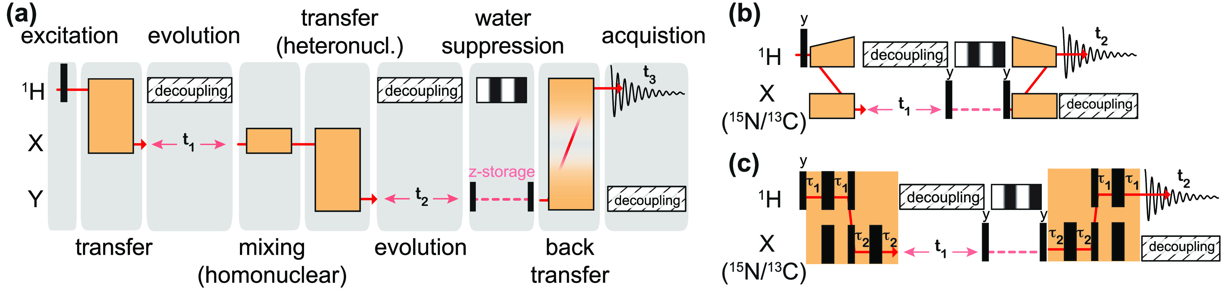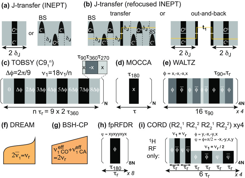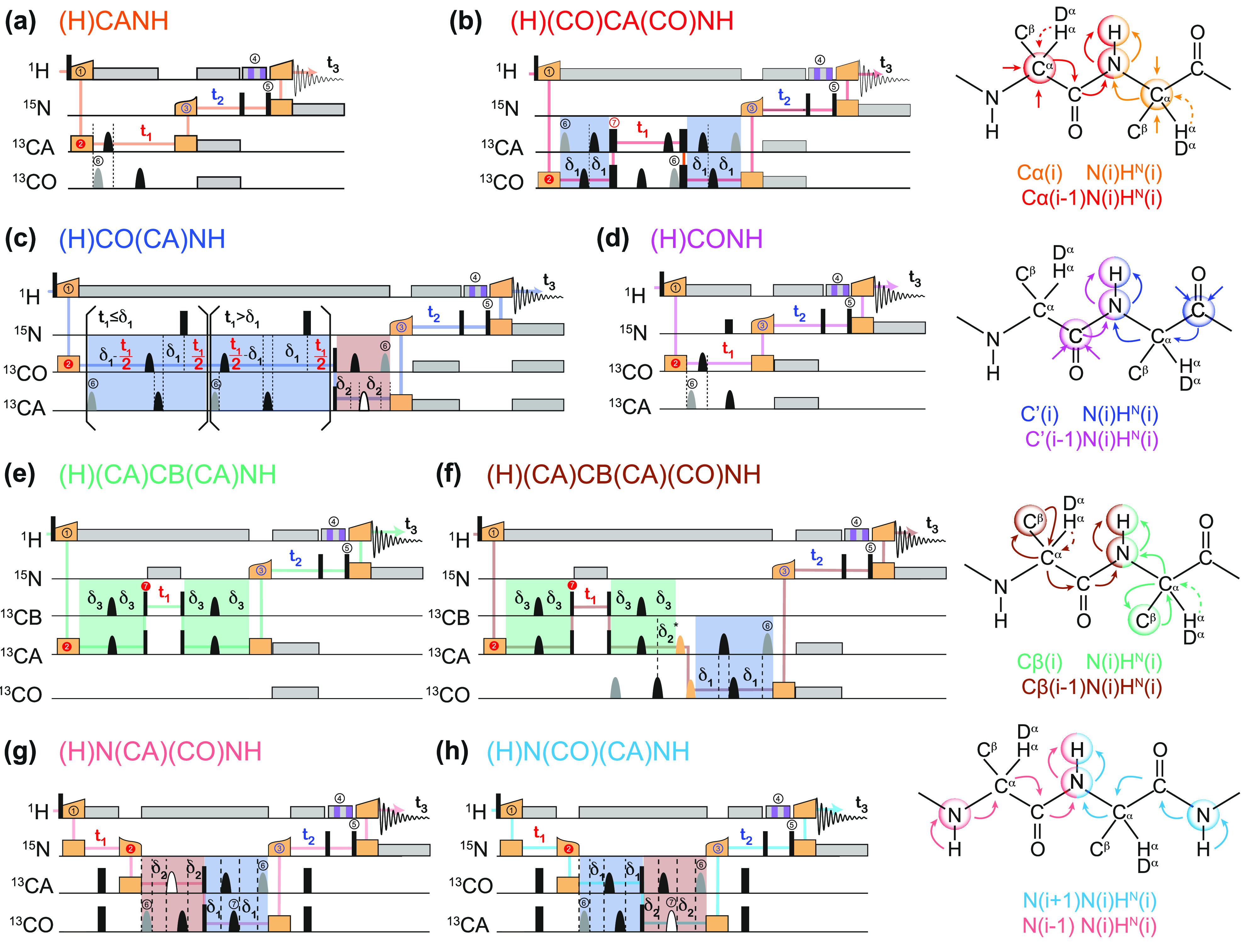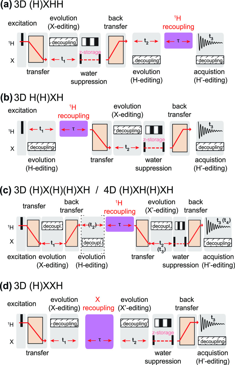All phases are applied along the x axis except for the pulses labeled with encircled numbers, for which the phases are cycled as follows: in all sequences, ① = , ② = , ③ = , ⑤ = y. In (b,e,f), ⑦ = x, and in (g,h), ⑦ = 8(x)8(y). Additionally, in (a−d,f,g,h), ⑥ = xy for suppression of undesired pathways. In (a−f), ϕ_rec = , and in (g,h), ϕ_rec =    . The full phase-cycle length of 8 for (a−f), and 16 (g,h) can be reduced to 4 and 8, respectively, with a minimal loss of quality. The phases of the MISSISSIPPI pulses ④ = xy are not cycled. Open and filled red (or blue) circles indicate phases which are respectively incremented or decremented for quadrature detection in t₁ (or t₂) according to the States-TPPI procedure. Off-resonance CP or selective pulses are performed with a fine stepwise phase modulation. The former require appropriate phase alignment either at the beginning or end of the CP pulse. In (b) and (c), ¹³C chemical shifts are evolved off-resonance; however, folding (aliasing) of resonance frequencies is avoided by t₁ time-proportional phase incrementation: Δφ = 360°ΔΩt₁ (in degrees), ΔΩ = Ω_C′/Cα – Δ_carrier, where Ω_C′/Cα are effective (requested) centers of either ¹³C′ or ¹³Cα bands. In (c), transfer time δ₁ is exploited for a constant-time evolution of ¹³C′ if t₁ < δ₁; otherwise, a real-time mode is used. Panels (a–f) were adapted with permission from ref (198) (copyright 2014 American Chemical Society) and panels (g−h) from ref (200) (copyright 2015 Springer Nature).

Figure 32

Representative 2D cross sections (strip plots) from (a) six H^N-detected 3D experiments providing intra- and inter-residue correlations to ¹³C′, ¹³Cα, and ¹³Cβ chemical shifts and (b) five Hα-detected 3D experiments correlating to ¹³C′, ¹⁵N, and ¹³Cβ. Chemical shift of the orthogonal (a) ¹⁵N or (b) ¹³Cα dimensions is indicated in each strip. Spectra were recorded on the deuterated (a) and nondeuterated (b) U-¹³C,¹⁵N-labeled samples of Acinetobacter phage 205 coat protein. Adapted with permission from (a) ref (198) (copyright 2014 American Chemical Society) and (b) ref (62) (copyright 2016 John Wiley & Sons).

Figure 33

Sensitivity of eight H^N-detected triple-resonance correlation experiments of Figure 31 relative to ¹H,¹⁵N CP-HSQC, measured in the first FIDs on a ¹³C,¹⁵N-labeled sample of microcrystalline maltose binding protein under 107 kHz MAS and at B₀ = 18.8 T.

Figure 34

Assignment of heterogeneous filaments of protein Tau.^, (a) Backbone walk using a pair of 4D nonuniformly sampled (H)CACONH and (H)COCANH spectra (black and pink contours, respectively), illustrated by a sequence of alternating 2D H^N/N and ¹³Cα/¹³C′ (orthogonal) cross sections. The strategy is supplemented by a 3D (H)N(CO)(CA)NH spectrum (gray contours). (b) Coherence transfer pathways of the three experiments used, sketched on a protein backbone. Adapted with permission from ref (199). Copyright 2016 Royal Society of Chemistry.

Figure 35

Representative 2D cross sections (strip plots) from two 3D experiments correlating ¹H,¹³C shifts of bonded nuclei to either ¹³C or ¹H chemical shifts of side-chain atoms within the same residue, recorded on a nondeuterated U-¹³C,¹⁵N-labeled sample of Acinetobacter phage 205 coat protein on a 23.5 T spectrometer at 100 kHz MAS. Cross-peaks of isoleucine-124 residue in 2D cross sections and in the ¹H,¹³C CP-HSQC are highlighted in red. Adapted with permission from ref (62). Copyright 2016 John Wiley & Sons.

Figure 36

(a) Coherence transfer scheme of a 4D HCCH experiment for ribose resonances of RNAs. CP and TOCSY transfers are depicted as solid and dotted arrows, respectively. (b) Representative ¹³C,¹H 2D planes from a 4D HCCH spectrum of a ¹³C,¹⁵N-labeled 26-nucleotide box C/D RNA complexed by L8Ae protein from Pyrococcus furiosus, recorded at 100 kHz MAS on a 18.8 T spectrometer. Intranucleotide correlations of G6, A18, and U20 detected on respective anomeric (H1′) protons (red contours) are overlaid on the ¹³C,¹H CP-HSQC spectrum (gray contours). Adapted with permission from ref (59). Copyright 2018 Royal Society of Chemistry.

Figure 37

Visualization of the spin density in a folded protein, PDB 6EKA, the β solenoid HELL-F. The first panel shows side-chains of a protein monomer (two layers in the β solenoid). The next panels depict spins within 4–10 Å of a β proton located in the core of the structure. Spins in b−f are colored white for protons, gray for carbon, blue for nitrogen, red for oxygen, and yellow for sulfur. Numbers in gray, black, and blue indicate the number of proton, carbon, and nitrogen spins, respectively, within the given distance.

Figure 38

Two examples of ¹H–¹H contacts particularly useful to define a protein fold. Panel (a) shows an example of helix–helix contact among methyl groups. Panel (b) shows an example of amide–amide contact that indicates a β-sheet arrangement.

Figure 39

Sequences employed to recouple ¹H–¹H dipolar interactions at the first (a,b) and second order of AHT (c,d). (a) Finite-pulse RFDR with xy8 phase cycling, a versatile scheme applied for a variety of conditions for broadband ¹H–¹H mixing, also in fully protonated samples. (b) DREAM mixing for selective recoupling within amide or methyl protons. (c,d) Sequences designed to enhance ¹H spin-diffusion through (c) ¹H spin-lock field (rotating-frame spin-diffusion) or (d) optimized RF irradiation of the X-nucleus (e.g., ¹⁵N), which affects (broadens) the ZQ linewidth of a coupled (bonded) proton. All schemes except AM-MIRROR use only ¹H RF irradiation. The spin operator (either polarization ¹H_z or transverse magnetization ¹H_xy) at the start of the mixing period is indicated.

Figure 40

Magnetization transfer schemes for obtaining secondary, tertiary, and quaternary structure information. (a–c) Amide-based proton–proton correlation, encoded as 4D or 3D variants. (d–f) H^C-based proton–proton correlations, encoded as 4D or 3D variants. Methyl contacts are shown; however, the general scheme also applies to methylene, aromatic, and other H^C moieties. (g) Carbon–carbon contacts. Heteronuclear contacts: (h) carbonyl carbon–proton contacts and (i) proton–carbon contacts; more generally, other heteronuclear contacts, such as proton–nitrogen or nitrogen–carbon, are also possible.

Figure 41

RF pulse schemes used for selective recoupling of ¹H–¹H interactions in fully protonated samples. (a) BASS-SD mixing with RF offset applied at the center of the amide proton frequency band (selection of other frequency bands, such as α or methyl protons is also possible). Panel (b) shows the SPR scheme, which is reminiscent of CN symmetry-based sequences, with a 90° pulse as a basic element (gray and black rectangles). SPR was further generalized for arbitrary phases (pSPR) and unrestricted phase incrementation, resulting in the identification of the MODIST sequence.

Figure 42

Selection of RF schemes used to recouple homonuclear (¹³C–¹³C or ¹⁵N–¹⁵N) dipolar interactions via second-order mechanisms involving a ¹H proxy spin. Panel (a) shows proton-assisted recoupling (PAR), which has been applied to monitor ¹³C–¹³C or ¹⁵N–¹⁵N distances. RF field strengths need to be empirically found with guidance from spin dynamics simulations but generally avoiding CP conditions. Panel (b) shows a CORD recoupling scheme, which has been used to record ¹³C–¹³C proximities, also in combination with RFDR (CORD-RFDR).

Figure 43

RF schemes employed for the detection of heteronuclear proximities. Panel (a) shows long-range cross-polarization, e.g., between remote ¹H and ¹³C′ spins. Panel (b) shows the basic element of REDOR, TEDOR, and TREDOR used for nitrogen–carbon and proton–carbon recoupling. This element is shown on a single channel, preferably the one of the rare (least abundant) nucleus, i.e., ¹⁵N, to avoid recoupling of homonuclear interactions. Additional pulses can be incorporated on the other channel to compensate for RF pulse imperfections.

Figure 44

(a) ¹H-detected measurement of ¹⁵N PREs from the comparison of ¹H,¹⁵N CP-HSQC spectra of Cu²⁺,Zn²⁺-SOD and Cu⁺,Zn²⁺-SOD. (b) ¹H-detected measurement of ¹H and ¹⁵N PCS from the comparison of ¹H,¹⁵N CP-HSQC spectra of Co²⁺-SOD and Zn²⁺-SOD (“E” - empty at the second binding site). Reproduced from ref (6). Copyright 2013 American Chemical Society.

Figure 45

Schematic RF irradiation schemes employed to record ¹H–¹H (a–c) or ¹³C–¹³C proximities (d) with ¹H detection. The asymmetric schemes (a) and (b) employ a heteronuclear (X) chemical shift evolution period before and after ¹H recoupling, respectively. Panel (c) shows an extended version with two heteronuclear (X) indirect dimensions, optionally augmented to a 4D experiment with a supplementary indirect ¹H evolution of the spin of origin. The RF diagram (d) is used to record heteronuclear distances via second-order recoupling.

Figure 46

Protein structures determined using proton-detected solid-state NMR (with corresponding PDB IDs in parentheses, if available), in the chronological order: GB1, SH3, ubiquitin (2L3Z), SOD (2LU5), M2 (2N70), bactofilin BacA (2N3D), AP205CP (5JZR), OmpG (5MWV), hCAII (6QEB), AlkL (6QWR), HELL-F amyloid (6EKA), and hVDAC1 (7QI2). Coordinates for GB1 and SH3 protein models were obtained from authors of respective publications.^,

Figure 47

¹H-detected long-range paramagnetic restraints used in the calculation of the solid-state NMR structure of SOD. In the different panel, bundles were calculated (a) without paramagnetic restraints, (b) with ¹⁵N and ¹³C PREs, (c) with ¹H, ¹⁵N, and ¹³C PCSs, and (d) with both PREs and PCSs. The Cu and Co ions are represented by violet and pink spheres, and the mean NMR structure is depicted as an aquamarine ribbon. Reproduced from ref (6). Copyright 2013 American Chemical Society.

Figure 48

Structural bundles of 10 lowest-energy conformers of fully protonated GB1 (a–d) and AP205CP (e–h) with specific long-range ¹H–¹H contacts indicated by purple lines: (b,f) between backbone amide protons; (c,g) between backbone amide and methyl protons of ILV residues, (d,h) between all protons. For AP205CP the symmetry-equivalent monomers are depicted in tan and cyan. Reproduced with permission from ref (111). Copyright 2016 National Academy of Sciences of the USA.

Figure 49

(a) Mixed labeling strategy used to detect intermolecular interactions in HELL-F amyloid based on a (1/1) [(U-¹H/¹⁴N)/(U-¹H^N/²H/¹⁵N)]-labeled sample. (b) Intermolecular distances based on a H···(H)NH experiment on (1/1) [(U-¹H/¹⁴N)/(U-¹H^N/²H/¹⁵N)]-labeled HELL-F. Adapted with permission from ref (215). Copyright 2021 National Academy of Sciences of the USA.

Figure 50

Flowchart of protein structure calculation based on proton-detected solid-state NMR experimental input. At the bottom, statistics of the GB1 structure calculation using UNIO-CANDID/CYANA are shown, illustrating the convergence of the calculation from cycles 1 to 7.

Figure 51

Proton–proton contact maps measured for AlkL. In (a), automatically generated contacts from peaks picked from the (H)NH(H)NH spectra. Contacts arising from one side of the spectrum diagonal are shown in red, whereas those from the other are shown in blue. In (b), the contact map of the final structure is shown, after resolution of ambiguities using CYANA, and including contacts from all spectra. Adapted with permission from ref (60). Copyright 2020 National Academy of Sciences of the USA.

Figure 52

“Hybrid” structures of TET2 aminopeptidase (PDB ID 6F3K) and bacteriophage SPP1 tail tube (PDB ID 6YQ5) determined using solid-state NMR ¹H–¹H contacts together with other structural methods (solution NMR and/or cryo-EM).

Figure 53

(a–c) Schematic representation of (b) spin relaxation caused by fluctuations of the anisotropic interactions and (c) direct measurement of scaled (motion-averaged) anisotropic interaction tensors, encoded in two chemical shift dimensions (a). Reproduced with permission from ref (27). Copyright 2021 Elsevier. (d) General block scheme of a ¹H-detected NMR experiment for site-specific measurement of heteronuclear spin relaxation, exchange, and/or anisotropic interaction recoupling for which the “relaxation/recoupling“ block is detailed in (e).

Figure 54

¹⁵N (a) and ¹³C (b) R₁ and R_1ρ relaxation rates calculated for variable correlation times and variable Larmor frequency (for R₁) or MAS frequency (for R_1ρ). Relaxation rates are calculated using the expressions derived from Redfield theory in ref (317) by assuming that ¹⁵N relaxation is driven by the dipolar interaction with a ¹H spin 1.02 Å away and by its CSA (170 ppm). For ¹³C relaxation, we considered a dipolar interaction with a ¹H spin 1.1 Å away and a CSA of 40 ppm. The density functions are assumed to follow the model-free formalism, with only the “internal” part of the Lipari–Szabo function and the order parameter S² fixed to 0.85.

Figure 55

¹⁵N R_1ρ relaxation–dispersion profiles for motions occurring at a typical time scale τ of 1 ms (blue) or 10 ns (red). The profiles are the sum of the rates calculated with Bloch–McConnell equations for a two-site exchange (with τ defined as 1/k_ex) and R_1ρ expression derived from Redfield theory for 40 kHz MAS (with τ being the correlation time).

Figure 56

(a) Side view of the proteasome assembly of Thermoplasma acidophilum with its molecular weight. The heptameric rings of the α-, β-, and 11S-subunits are colored in green, red, and white, respectively. One α-subunit is highlighted in orange. (b) Resonance assignment of the proteasome α-subunit within the 1.1 MDa 11S-α₇β₇β₇α₇-11S complex. Reprinted with permission from ref (354). Copyright 2013 John Wiley & Sons.

Figure 57

CP (H)PH correlation spectrum recorded on a sedimented complex of DnaB with ADP:AlF₄^– and DNA at 105 kHz MAS. Correlations between the phosphate groups and ADP or DNA are highlighted in green and light red/purple, respectively. Reproduced with permission from ref (364). Copyright 2021 Springer Nature.

Figure 58

(a) Soluble FcRn_ECD (42 kDa) was sedimented by ultracentrifugation directly into a 0.7 mm MAS NMR rotor. (b) CSPs upon UCB-FcRn-303 binding to FcRn_ECD as observed in 2D planes of 3D (H)CANH spectra with (black) and without (blue) the ligand. (c) CSPs are mapped on the FcRn_ECD diprotomer structure in complex with UCB-FcRn-303 (red). In (d), the FcRn_ECD crystal structure is shown in cartoon representation with β2m in green and dark gray and the α-chain molecules in blue and light gray. Reprinted with permission from ref (232). Copyright 2018 PLoS.

Figure 59

2D cross sections (left) of a 3D H(H)CH-RFDR spectrum acquired on U-[¹⁵N, ¹³C] proteorhodopsin in lipids at 100 kHz MAS at 305 K and 23.5 T, with ¹H–¹H correlations assigned to intra/interhelical and helix-retinal contact cofactor, as depicted in the schematic 3D structure of the protein (right). Reprinted from ref (228). Copyright 2017 American Chemical Society.

Figure 60

(a) Negative-stain electron microscopy images of heterogeneous paired helical filaments of protein Tau and (b) their assigned ¹H,¹⁵N CP-HSQC spectrum showing significant inhomogeneous line broadening. (c,d) Pictorial interpretation of how the NMR shifts from invariant and variable residues may originate in the fibril building block: (c) secondary structure (β-strand or loop/kink, as derived from ¹³C secondary chemical shifts) is comparable among different batches of samples; however, ¹⁵N chemical shifts of many regions (“non-blue”) vary between different fibrils; (d) variability of the local chemical environment, including H-bond architecture, including shearing (top), twisting (middle), and bending of β-sheets (bottom). Reprinted from ref (63). Copyright 2017 American Chemical Society.

Figure 61

HELL-F(209–277) amyloid fold presents strong similarity with HET-s (218–289), while the two prion domains lack in vivo cross-seeding. (a) Backbone structural alignment of the MAS NMR structures of the HELL-F (in blue) and HET-s (in yellow) prion-forming domains. (b,c) Four cartoons representing the hydrophobic triangular core of amyloid fibrils formed by the successively stacked pseudorepeats—R1 (left) and R2 (right)—of HELL-F (b) and HET-s (c). Hydrophobic residues are shown in white, acidic residues in red, basic residues in blue, and others in green. Reprinted with permission from ref (215). Copyright 2021 National Academy of Sciences of the USA.

Figure 62

Measurement of site-specific proximity to mobile small molecules, water, lipids, and cholesterol. (a) Water-exposed residues in KcsA are highlighted based on a (H)NH spectrum after the sample is washed in acidic buffer. Proximity to water was recorded in the same study via H(H)N and H(H)CC spectra. Reprinted from ref (374). Copyright 2014 American Chemical Society. (b) Selected strips from a 4D H(H)(N)CANH spectrum highlighting cross-peaks to water and lipid moieties. Reprinted with permission from ref (375). Copyright 2019 John Wiley & Sons. Panel (c) shows cholesterol docked to the structure of VDAC, in agreement with the measured proximity to nearby residues as determined by transfer from the protons of cholesterol in a H(H)NH spectrum. Adjacent hydrophobic side-chains that form grooves on the outside of the protein are labeled. Reprinted with permission from ref (376). Copyright 2021 Springer Nature. (d) Sites of water exposure are mapped onto the structure of GLPG, based on a H(H)NH spectrum, shown in red. Reproduced from ref (230). Copyright 2019 American Chemical Society.

Figure 63

(a) Overlaid 2D ¹⁵N–¹H projections of 3D (H)CANH spectrum of the NS5A-AHD1 protein in the presence of Lu³⁺-DPPE (blue) or Gd³⁺-DPPE lipids (red) mixed with PC/Chol lipids. (b) Membrane orientation of NS5A-AHD1. PREs are color-coded on the homology models based on X-ray structure of D1 and HA. Blue-gray-red qualification shows increasing PRE. Reprinted with permission from ref (109). Copyright 2021 John Wiley & Sons.

Figure 64

(a) Representation of conformational dynamics in hCAII. The protein backbone is represented as a cylinder, where thickness and color (gray to red) highlight areas undergoing microsecond conformational exchange in the active site loop, assessed by ¹⁵N relaxation–dispersion experiments. (b–e) Effect of ligand binding on the exchange motions of hCAII sensed by T198 backbone and N67 side-chain ¹⁵N spin. The top row shows the free form, whereas the bottom row shows the dorzolamide-bound form. Reprinted with permission from ref (339) (copyright 2019 American Chemical Society) and from ref (27) (copyright 2021 Elsevier).

Figure 65

NMR spectra of Co-SOD acquired at 100 kHz MAS on a 500 MHz spectrometer. (a) ¹H spectrum (1D spin–echo), (b,c) 2D ¹H, ¹³C, and ¹H, ¹⁵N TEDOR correlation spectra, acquired without (black) and with (magenta) spin magnetization exchange between ¹H nuclei close in space. (d) Overlay of Zn²⁺ site in 10 protein chains of the single-crystal X-ray structure of SOD 1, illustrating the crystallographic uncertainty in the metal coordination geometry and (e) NMR ensemble of structures of the Co²⁺ complex of Co-SOD. Schematic representation of the metal site (f) in the X-ray diffraction ensemble and (g) in the NMR ensemble. Reprinted from ref (385). Copyright 2020 American Chemical Society.

Figure 66

Revealing hydrogen bonding and protonation states. (a) N–H···N hydrogen bond is detected through measurement of a ^2HJ_NN coupling (blue and green) for H37 of Influenza A M2. In black and red, this hydrogen bond is broken upon addition of the inhibitor rimantadine. Reproduced from ref (389). Copyright 2020 American Chemical Society. (b) Long-range CP transfers were used in the NH spectra to identify tautomer states of histidine, as well as a hydroxyl proton hydrogen bonded to a histidine side-chain nitrogen. These histidine residues are at the heart of active chemistry in carbonic anhydrase. Reprinted with permission from ref (271). Copyright 2019 John Wiley & Sons. (c) Low- and high-temperature spectra were used to identify the chemical shift of a water proton hydrogen-bonded to a histidine side-chain nitrogen in the M2 protein from Influenza A. Reproduced with permission from ref (391). Copyright 2021 John Wiley & Sons. (d) Selective TEDOR sequence was used to identify tautomer states in the C-terminal domain of the HIV capsid protein with SP1 using fractional deuteration. Reprinted with permission from ref (392). Copyright 2021 Frontiers Media SA.

Figure 67

(a) ¹⁵N rotating-frame ssNMR relaxation rates (R_1ρ) that report on slow molecular motions in wild-type (WT) KcsA and mutants E71A, E71I, and E71Q; signal decay curves are shown for selected filter residues. The illustrations show the site-resolved selectivity filter dynamics. The size of the spheres corresponds to the R_1ρ relaxation rates. (b) 2D ¹H–¹⁵N spectra of E71A in protonated (red) and deuterated (gray) buffers showing the fast exchange of Y78, together with illustrations of the NMR-derived water cavity size in WT KcsA and mutants. Reprinted with permission from ref (231). Copyright 2019 Springer Nature.

Figure 68

Lipid II–nisin complex in cellular membranes. (a) Comparison of ¹H-detected 2D ¹H–¹⁵N spectra of lipid II-bound nisin in native M. flavus membranes (magenta) and in DOPC (cyan). The gray spectrum shows nisin nonspecifically bound to DOPG/DOPC liposomes (7:3 ratio) in the absence of lipid II. (b) Membrane arrangement of the nisin/lipid II topology as seen by MAS NMR. Plastic residues that are required to adapt to the bacterial target membrane are highlighted with red circles. Residues that showed ¹H/²H exchange are colored in blue and align the pore lumen. The C-terminus is dynamically disordered and resides at the water–membrane interface. Reprinted with permission from ref (397). Copyright 2018 Springer Nature.

Figure 69

Region of α-resonances of ¹H–¹³C CP-HSQC spectrum recorded on a sample of microcrystalline protein GB1 at natural abundance (implying also no deuteration), in a 0.7 mm rotor spun at 100 kHz on a 23.5 T spectrometer. Microcrystals were doped (impregnated) with paramagnetic Cu(II) ions to increase scan recycling and thus boost sensitivity. Note that no heteronuclear decoupling was needed during acquisition, and that ¹³C lines are free from homonuclear scalar couplings.

References

-
- Hologne M.; Chevelkov V.; Reif B. Deuterated Peptides and Proteins in MAS Solid-State NMR. Prog. Nucl. Magn. Reson. Spectrosc. 2006, 48, 211–232. 10.1016/j.pnmrs.2006.05.004. - DOI
- Reif B. In Protein NMR Techniques; Shekhtman A., Burz D. S., Eds.; Humana Press: Totowa, NJ, 2012; pp 279–301.
Publication types
MeSH terms
Substances
LinkOut - more resources
Full Text Sources