Reinforcement learning and Bayesian inference provide complementary models for the unique advantage of adolescents in stochastic reversal

Abstract

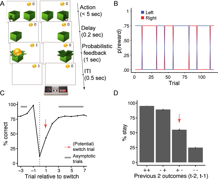
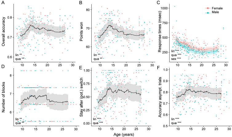
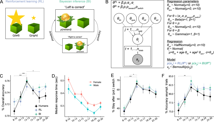
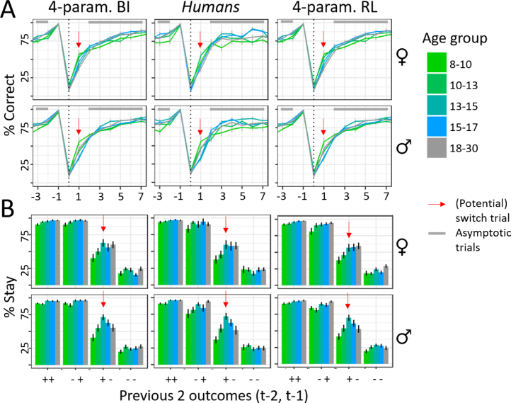
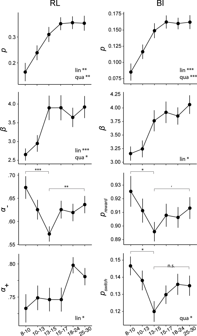
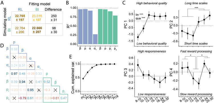
During adolescence, youth venture out, explore the wider world, and are challenged to learn how to navigate novel and uncertain environments. We investigated how performance changes across adolescent development in a stochastic, volatile reversal-learning task that uniquely taxes the balance of persistence and flexibility. In a sample of 291 participants aged 8-30, we found that in the mid-teen years, adolescents outperformed both younger and older participants. We developed two independent cognitive models, based on Reinforcement learning (RL) and Bayesian inference (BI). The RL parameter for learning from negative outcomes and the BI parameters specifying participants' mental models were closest to optimal in mid-teen adolescents, suggesting a central role in adolescent cognitive processing. By contrast, persistence and noise parameters improved monotonically with age. We distilled the insights of RL and BI using principal component analysis and found that three shared components interacted to form the adolescent performance peak: adult-like behavioral quality, child-like time scales, and developmentally-unique processing of positive feedback. This research highlights adolescence as a neurodevelopmental window that can create performance advantages in volatile and uncertain environments. It also shows how detailed insights can be gleaned by using cognitive models in new ways.

Keywords: Adolescence; Bayesian inference; Computational modeling; Development; Non-linear changes; Reinforcement learning; Volatility.

Fig. 1

(A) Task design. On each trial, participants chose one of two boxes, using the two red buttons of the shown game controller. The chosen box either revealed a gold coin (left) or was empty (right). The probability of coin reward was 75% on the rewarded side, and 0% on the non-rewarded side. (B) The rewarded side changed multiple times, according to unpredictable task switches, creating distinct task blocks. Each colored line (blue, red) indicates the reward probability ($p\left(reward\right)$) of one box (left, right) at a given trial, for an example session. (C) Average human performance and standard errors, aligned to true task switches (dotted line; trial 0). Switches only occurred after rewarded trials (Section 4.3), resulting in performance of 100% on trial -1. The red arrow shows the switch trial, gray bars show trials included as asymptotic performance. (D) Average probability of repeating a previous choice (“stay”) as a function of the two previous outcomes ($t-2$, $t-1$) for this choice (“$+$”: reward; “–”: no reward). Error bars indicate between-participant standard errors. Red arrow highlights potential switch trials like in part C, i.e., when a rewarded trial is followed by a non-rewarded one, which—from participants’ perspective—is consistent with a task switch. (For interpretation of the references to color in this figure legend, the reader is referred to the web version of this article.)

Fig. 2

Task performance across age. Each dot shows one participant, color denotes sex. Lines show rolling averages, shades the standard error of the mean. The stars for “lin”, “qua”, and “sex” denote the significance of the effects of age, squared age, and sex on each performance measure, based on the regression models in Table 1 (* $p<.05$, ** $p<.01$, *** $p<.001$) (A) Proportion of correct choices across the entire task (120 trials), showing a peak in adolescents. The non-linear development was confirmed by the quadratic effect of age (“qua”; Table 1), and the U-shape by the significant two-line analysis (Table 2). (B) (Corrected) number of points won in the game (Section 4.4), showing a peak in adolescents, confirmed by the quadratic effect of age and significant two-line analysis. (C) Median response times on correct trials. Regression coefficients differed significantly between males and females; rolling averages are hence shown separately. The performance peak occurred after adolescence. (D) (Corrected) number of blocks completed by each participant (Section 4.4), showing a quadratic effect of age. (E) Fraction of trials on which each participant “stayed” after a (potential, “pot.”) switch trial (red arrows in Fig. 1C and D), showing a peak in adolescents and quadratic age effect. (F) Accuracy on asymptotic trials (horizontal gray bars in Fig. 1C), also showing a peak in adolescents and quadratic age effect.

Fig. 3

(A) Conceptual depiction of the RL and BI models. In RL (left), actions are selected based on learned values, illustrated by the size of stars ($Q\left(left\right)$, $Q\left(right\right)$). Values are calculated based on previous outcomes (Section 4.5.1). In BI (right), actions are selected based on a mental model of the task, which differentiates different hidden states (“Left is correct”, “Right is correct”), and specifies the transition probability between them ($p\left(switch\right)$) as well as the task’s reward stochasticity ($p\left(reward\right)$). The sizes of the two boxes illustrate the inferred probability of being in each state (Section 4.5.2). (B) Hierarchical Bayesian model fitting. Box: RL and BI models had free parameters ${\theta }^{RL}$ and ${\theta }^{BI}$, respectively. Individual parameters ${\theta }_j$ were based on group-level parameters ${\theta }_{sd}$, ${\theta }_{int}$, ${\theta }_{lin}$, and ${\theta }_{qua}$ in a regression setting (see text to the right). For each model, all parameters were simultaneously fit to the observed (shaded) sequence of actions $a_{jt}$ of all participants $j$ and trials $t$, using MCMC sampling. Right: We chose uninformative priors for group-level parameters; the shape of each prior was based on the parameter’s allowed range. For each participant $j$, each parameter $\theta$ was sampled according to a linear regression model, based on group-wide standard deviation ${\theta }_{sd}$, intercept ${\theta }_{int}$, linear change with age ${\theta }_{lin}$, and quadratic change with age ${\theta }_{qua}$. Each model (RL or BI) provided a choice likelihood $p\left(a_{jt}\right)$ for each participant $j$ on each trial $t$, based on individual parameters ${\theta }_j$. Action selection followed a Bernoulli distribution (for details, see Sections 4.5.3 and 6.2.2). (C)–(F) Human behavior for the measures shown in Fig. 2, binned in age quantiles. (C), (E), and (F) also show simulated model behavior for model validation, verifying that models closely reproduced human behavior and age differences.

Fig. 4

Model validation, comparing simulated behavior of the winning 4-parameter BI model (left column), humans (middle column), and the winning 4-parameter RL model (right column). Both models show excellent fit, evident in the fact that simulated behavior is barely distinguishable from human behavior (Appendix 6.3.6). (A) Behavior in trials surrounding a real switch of the correct choice ($t=0$) shows that both models capture well the quick adaptation for all groups. Colors refer to age groups, red arrows show switch trials, gray bars trials of asymptotic performance, like in Fig. 1C. (B) Stay probability in response to outcomes 1 and 2 trials back, like in Fig. 1D. Both models capture well the empirical pattern of switching behavior.

Fig. 5

Fitted model parameters for the winning RL (left column) and BI model (right), plotted over age. Stars in combination with “lin” or “qua” indicate significant linear (“lin”) and quadratic (“qua”) effects of age on model parameters, based on the age-based fitting model (Section 4.5.3). Stars on top of brackets show differences between groups, as revealed by t-tests conducted within the “age-less fitting model” (Section 4.5.3; suppl. Tables 13 and 14). Dots (means) and error bars (standard errors) show the results of the age-less fitting model, providing an unbiased representation of individual fits.

Fig. 6

Relating RL and BI models. (A) Model recovery. WAIC scores were worse (larger; lighter colors) when recovering behavior that was simulated from one model (row) using the other model (column), than when using the same model (diagonal), revealing that the models were discriminable. The difference in fit was smaller for BI simulations (bottom row), suggesting that the RL model captured BI behavior better than the other way around (top row). (B) Variance of each parameter explained by parameters and interactions of the other model (“$R^2$”), estimated through linear regression. All four BI parameters (green) were predicted almost perfectly by the RL parameters, and all RL parameters except for ${\alpha }_{+}$ (RL) were predicted by the BI parameters. (D) Spearman pairwise correlations between model parameters. Red (blue) hue indicates negative (positive) correlation, saturation indicates correlation strength. Non-significant correlations are crossed out (Bonferroni-corrected at $p=0.00089$). Light-blue (teal) letters refer to RL (BI) model parameters. Light-blue/teal-colored triangles show correlations within each model, remaining cells show correlations between models. (C) & (E) Results of PCA on model parameters (Section 4.5.5). (C) Age-related differences in PC1–4: As revealed by PC-based model simulations (Appendix 6.3.11), PC1 reflected overall behavioral quality. It showed rapid development between ages 8–13, which were captured by linear (“lin”) and quadratic (“qua”) effects in a regression model. PC2 captured a step-like transition from shorter to longer updating time scales at age 15. PC3 showed no significant age effects. PC4 captured the variance in ${\alpha }_{+}$ and differed between adolescents 15–17 and both 8–13 year olds and adults. PC2 and PC4 were analyzed using t-tests. * $p<.05$; ** $p<.01$, *** $p<.001$. (E) Cumulative variance explained by all principal components PC1–8. The first four components analyzed in more detail captured 96.5% of total parameter variance. (For interpretation of the references to color in this figure legend, the reader is referred to the web version of this article.)

References

1. Adleman N., Kayser R., Dickstein D., Blair R., Pine D., Leibenluft E. Neural correlates of reversal learning in severe mood dysregulation and pediatric bipolar disorder. J. Am. Acad. Child Adolesc. Psychiatry. 2011;50:1173–1185.e2. doi: 10.1016/j.jaac.2011.07.011. - DOI - PMC - PubMed
1. Albert D., Chein J., Steinberg L. The teenage brain: Peer influences on adolescent decision making. Curr. Direct. Psychol. Sci. 2013;22(2):114–120. doi: 10.1177/0963721412471347. - DOI - PMC - PubMed
1. Bartolo R., Averbeck B.B. Prefrontal cortex predicts state switches during reversal learning. Neuron. 2020;106(6):1044–1054.e4. doi: 10.1016/j.neuron.2020.03.024. - DOI - PMC - PubMed
1. Bates D., Mächler M., Bolker B., Walker S. Fitting linear mixed-effects models using lme4. J. Stat. Softw. 2015;67(1):1–48. doi: 10.18637/jss.v067.i01. - DOI
1. Bernardo J.M., Smith A.F.M. John Wiley & Sons; 2009. Bayesian Theory. Google-Books-ID: 11nSgIcd7xQC.
Publication types