Training a spiking neuronal network model of visual-motor cortex to play a virtual racket-ball game using reinforcement learning

Abstract

Recent models of spiking neuronal networks have been trained to perform behaviors in static environments using a variety of learning rules, with varying degrees of biological realism. Most of these models have not been tested in dynamic visual environments where models must make predictions on future states and adjust their behavior accordingly. The models using these learning rules are often treated as black boxes, with little analysis on circuit architectures and learning mechanisms supporting optimal performance. Here we developed visual/motor spiking neuronal network models and trained them to play a virtual racket-ball game using several reinforcement learning algorithms inspired by the dopaminergic reward system. We systematically investigated how different architectures and circuit-motifs (feed-forward, recurrent, feedback) contributed to learning and performance. We also developed a new biologically-inspired learning rule that significantly enhanced performance, while reducing training time. Our models included visual areas encoding game inputs and relaying the information to motor areas, which used this information to learn to move the racket to hit the ball. Neurons in the early visual area relayed information encoding object location and motion direction across the network. Neuronal association areas encoded spatial relationships between objects in the visual scene. Motor populations received inputs from visual and association areas representing the dorsal pathway. Two populations of motor neurons generated commands to move the racket up or down. Model-generated actions updated the environment and triggered reward or punishment signals that adjusted synaptic weights so that the models could learn which actions led to reward. Here we demonstrate that our biologically-plausible learning rules were effective in training spiking neuronal network models to solve problems in dynamic environments. We used our models to dissect the circuit architectures and learning rules most effective for learning. Our model shows that learning mechanisms involving different neural circuits produce similar performance in sensory-motor tasks. In biological networks, all learning mechanisms may complement one another, accelerating the learning capabilities of animals. Furthermore, this also highlights the resilience and redundancy in biological systems.

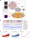
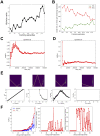
Fig 1. Constructing a feedforward model of visual-motor cortex that learns to play the racket-ball game.

A) Schematic of the closed-loop feedforward visual/motor circuit model interfaced with the racket-ball game. Visual areas receive inputs from the pixelated image frames of the racket-ball game, downstream activating association and motor areas. An action is generated after comparing firing rates of EMDOWN and EMUP excitatory motor populations over an interval. Each action delivers a reward to the model driving STDP-RL learning rules. B) Raster plot shows the spiking activity of different populations of neurons during a training episode (vertical axis is neuron identity and horizontal axis is time; each dot represents a single action potential from an individual neuron). Patterned activation of early visual neurons (i.e. diagonal lines in raster plots) indicate for example, the ball traversing the court from side to side. These patterns are visible because the early visual neurons were arranged topographically with increasing neuron number. C) Firing rates of excitatory motor neuron populations EMUP and EMDOWN in the feedforward model increase over the course of training. The firing rates were binned for ball trajectories (beginning when the ball is at the extreme left side of the court and ends when the ball hits or misses the racket on the right side of the court). D) The average weight change of synaptic input onto EMUP and EMDOWN sampled over 20 training episodes tends to increase with learning, indicating the network tends to produce rewarding behavior.

Fig 2

Spike-timing dependent reinforcement learning framework: A) An exponentially-decaying synaptic eligibility trace (ET) is triggered after postsynaptic neuron firing within a short time window after presynaptic neuron firing. If a reward or punishment signal is delivered while ET>0, synaptic weight is potentiated or depressed proportional to ET. B) IRP delivers rewards to the model for each action it takes based on whether the action moved the racket towards the projected location of the ball for a hit or away. C) Three different RL versions used in this study (V visual; A Association; M Motor areas): non-targeted RL, all motor neurons receive ET; targeted RL, motor neurons which contributed to the action receive ET and motor neurons in population for the other directions receive negative ET; retrograde targeted RL as in targeted RL but middle/hidden layer synaptic connections also receive ET, with ET amplitude reduction based on number of back-tracked connections.

Fig 3. The performance of the feedforward spiking neuronal network model using spike-timing dependent RL improved over repeated training episodes.

A) The cumulative Hit/Miss ratio at the end of each 500 sec training episode is plotted as a function of training episodes. B) The total number of Hits and Miss at the end of each training episode is plotted as a function of training episodes. C, D) The temporal evolution of performance for the training episodes 18 and 19. E, F) Summary of learning performance for different ball trajectories. E) Four example ball trajectories are shown together with the performance over repeats. The upper panels show the average of all Input Images corresponding to a unique ball trajectory and the performance is shown in lower panels. These example ball trajectories show visual input specific model learning. For some ball trajectories (e.g. first example), the model-controlled-racket always hits the ball, whereas for some other ball trajectories (e.g. fourth example), it never hits the ball. In the second example, the model-controlled-racket missed the ball only after 15 repetitions. In the third example, the performance first improved, followed by a big drop. F) The left panel: median and maximum performance for unique ball trajectories. The middle panel: number of repeats at which the model had peak performance. The right panel: relative number of repeats at which the model had peak performance. This indicates that for some ball trajectories (# 30–32), the model performed at peak without any training and the training only reduced the performance of the model. For some ball trajectories (# 0–5), the model could not learn to hit the ball. This also shows that for some ball trajectories (see the trajectories with relative # of repeats for max. Hit/Miss values between 0.2 and 0.8), the model first learns to hit the ball and then forgets, whereas for a few ball trajectories (see the trajectories with relative # of repeats for max. Hit/Miss values 0.8 or above), the model did not forget how to hit the ball until the end of all training sessions.

Fig 4. The feedforward spiking neuronal network model sustained its performance after learning.

A) The bar plot shows the mean (n = 6) performance (Hit/Miss) of the model before training (using initial weights), after training episode 18 and after training episode 19. For each condition, 6 different initial positions of the racket and the ball were used to evaluate and compare the performance of the model after learning. Each simulation was run for the duration of 500 sec. B) The temporal evolution of the cumulative performance (Hit/Miss) for the model before learning (using initial weights for synaptic connections). The traces in different colors show performance for different initial positions of the ball and the racket. C) Same as in B using fixed weights for synaptic connections after training episode 18. D) Same as in C using fixed weights for synaptic connections after training episode 19. E, F) Two example ball trajectories where the model showed robust and sustained learning after training episodes 18 (middle) and 19 (right) as compared to before learning (left) G) The peak (best cumulative Hit/Miss during repeats) and the median (median of cumulative Hit/Miss during repeats) performance for all different ball trajectories is summarized for the model before training (left) and after training episodes 18 (middle) and 19 (right).

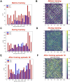
Fig 5. The feedforward spiking neuronal network model learned to perform better for the ball trajectories towards the center compared to the ball trajectories towards the corners of the court.

The bar plots in A,C and E show the number of ‘Hits’ and the number of ‘Misses’ against the ball’s vertical position (ypos) when crossing the racket for the model before, during and after training respectively. The heatmaps in B, D and F show the probability of a correct move for each ball location in the court for the model before, during and after training respectively. The color at each pixel in the heatmaps shows the probability of correct action when the ball was at that location based on the projected Hit coordinates (when the action is the same as the proposed action). The white pixels represent the locations never parsed by the ball. Similarly the white space on the right side of each heatmap indicates the region, where no proposed action was available for the model racket (p(correct move) = NaN) as the ball had already passed the racket on the right side of the court.

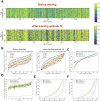
Fig 6. After training, the dynamics of motor neurons taking part in action generation change.

A) The heat maps show how often each EMUP neuron was among 70% most active neurons during repeated occurance of the same ball trajectory before training (upper heatmap) and after training episode 18 (lower heatmap). Note that the neuron ids are the same in both heatmaps but input seq ids may vary. B) The plot shows how often each EMUP neuron was among 70%, 60%, 50% and 40% most active neurons during repeated occurance of the same ball trajectory before training (left: BT) and after training episode 18 (right: AT18). Note that the neuron ids are sorted using top 70% neuron indices. C) Comparing the average probability of each motor (EMUP) neuron being among 70% most active neurons before and after training episodes 18 and 19. D) The plot compares the percentage of times a motor (EMUP) neuron actively contributed to action generation. After training, the contribution of each motor (EMUP) neuron in action generation increased proportionally (with some variability) to the contribution before training. E) The plot compares how many times at least 1 EMUP neuron was involved in action generation before and after training. Before training, at least 1 EMUP neuron was active for 28% of actions generated. After training, at least 1 EMUP neuron was active for 42% of actions generated. F) The plot compares how many times at least 1 motor neuron (either EMUP or EMDOWN) was involved in action generation before and after training. Before training, at least 1 motor neuron was active for 53% of actions generated. After training, at least 1 motor neuron was active for 83% of actions generated.

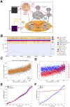
Fig 7. The synaptic weights of the recurrent spiking neuronal network model were adjusted to ensure reliable transmission of the input information across all network areas.

A) The schematic shows the racket-ball game interfaced with the recurrent model of visual and motor areas. B) Raster plot showing the spiking activity of different populations of neurons during a training episode. C) Firing rates of motor neuron populations ‘EMUP’ and ‘EMDOWN’ in the recurrent model. D) same as in C for ‘EA’ and ‘EA2’. The firing rates in C and D were binned for ball trajectories (each ball trajectory from the extreme left to the right side of the court where the ball hits or misses the racket). E) Average weight change of synaptic input onto ‘EMUP’ and ‘EMDOWN’ sampled over 40 training episodes. F) same as in E for ‘EA’ and ‘EA2’ sampled over 40 training episodes.

Fig 8. The recurrent model with sparse rewards shows sustained performance after learning.

A) cumulative performance at the end of 40 training episodes. B) Cumulative Hits and Misses at the end of 40 training episodes. C) Temporal evolution of performance during training episode 31. D) Comparing performance of the model using weights from the end of training episode 31 (right) with the performance of the model before training (using initial weights; left). For both cases, the simulation was repeated 9 times each with different initial positions of the ball and the racket and the performance of each simulation is shown using black dots. The bar plot shows the average of those 9 simulations. E, F) Learning by the model is shown using two example ball trajectories. The left panels show the model’s performance for the repeated encounter of the ball trajectory when simulated using the initial synaptic weights (before learning). The right panels show the same as in the left panels but using the synaptic weights at the end of training episode 31 (peak performance AT in F is 3).

Fig 9. After training the recurrent model with sparse rewards, the dynamics of motor neurons taking part in action generation change.

A) The heat maps show how often each EMUP neuron was among 70% most active neurons during repeated occurance of the same ball trajectory before training (upper heatmap) and after training episode 31 (lower heatmap). Note that the neuron ids are the same in both heatmaps but input seq ids may vary. B) The plot shows how often each EMUP neuron was among 70%, 60%, 50% and 40% most active neurons during repeated occurance of the same ball trajectory before training (left) and after training episode 31 (right). Note that the neuron ids are sorted using top 70% neuron indices. C) Comparing the average probability of each motor (EMUP) neuron being among 70% most active neurons before and after training episode31. D) The plot compares the percentage of times a motor (EMUP) neuron actively contributed to action generation. After training, the contribution of each motor (EMUP) neuron in action generation increased proportionally (with some variability) to the contribution before training. E) The plot compares how many times at least 1 EMUP neuron was involved in action generation before and after training. Before and after training, at least 1 EMUP neuron was active for 55% of actions generated. F) The plot compares how many times at least 1 motor neuron (either EMUP or EMDOWN) was involved in action generation before and after training. Before training, at least 1 motor neuron was active for 92% of actions generated. After training, at least 1 motor neuron was active for 93% of actions generated.

References

1. Van Hasselt H, Guez A, Silver D. Deep reinforcement learning with double q-learning. Proceedings of the AAAI conference on artificial intelligence. 2016. https://ojs.aaai.org/index.php/AAAI/article/view/10295
1. Sutton RS, Barto AG. Reinforcement learning: An introduction. MIT press; Cambridge; 1998. http://www.cell.com/trends/cognitive-sciences/pdf/S1364-6613(99)01331-5.pdf
1. Witty S, Lee JK, Tosch E, Atrey A, Littman M, Jensen D. Measuring and Characterizing Generalization in Deep Reinforcement Learning. arXiv [cs.LG]. 2018. http://arxiv.org/abs/1812.02868
1. Wang Z, Schaul T, Hessel M, Hasselt H, Lanctot M, Freitas N. Dueling Network Architectures for Deep Reinforcement Learning. In: Balcan MF, Weinberger KQ, editors. Proceedings of The 33rd International Conference on Machine Learning. New York, New York, USA: PMLR; 2016. pp. 1995–2003.
1. Mnih V, Kavukcuoglu K, Silver D, Rusu AA, Veness J, Bellemare MG, et al.. Human-level control through deep reinforcement learning. Nature. 2015;518: 529–533. doi: 10.1038/nature14236 - DOI - PubMed
Publication types