Degron masking outlines degronons, co-degrading functional modules in the proteome

Abstract

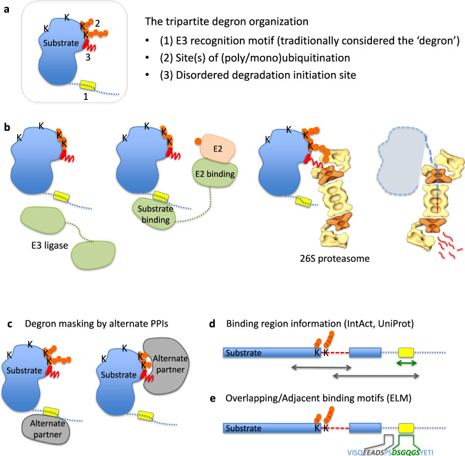
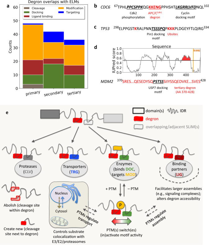
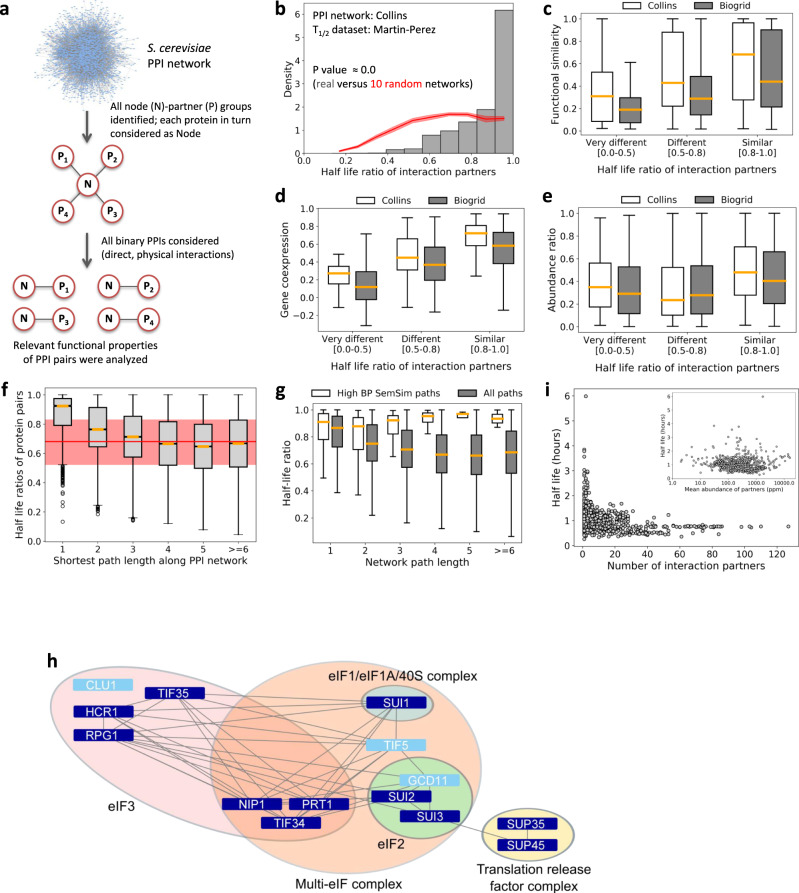
Effective organization of proteins into functional modules (networks, pathways) requires systems-level coordination between transcription, translation and degradation. Whereas the cooperation between transcription and translation was extensively studied, the cooperative degradation regulation of protein complexes and pathways has not been systematically assessed. Here we comprehensively analyzed degron masking, a major mechanism by which cellular systems coordinate degron recognition and protein degradation. For over 200 substrates with characterized degrons (E3 ligase targeting motifs, ubiquitination sites and disordered proteasomal entry sequences), we demonstrate that degrons extensively overlap with protein-protein interaction sites. Analysis of binding site information and protein abundance comparisons show that regulatory partners effectively outcompete E3 ligases, masking degrons from the ubiquitination machinery. Protein abundance variations between normal and cancer cells highlight the dynamics of degron masking components. Finally, integrative analysis of gene co-expression, half-life correlations and functional relationships between interacting proteins point towards higher-order, co-regulated degradation modules ('degronons') in the proteome.

Fig. 1. Schematic of tripartite degrons and their masking by PPIs.

a Tripartite degron organization, and, (b) schematic overview of how each of the degron components mediates specific steps in substrate selection and degradation in the UPS (adapted from Guharoy et al.). Firstly, E3 ligases target specific substrates via primary degrons, followed by ubiquitination of single (or multiple, neighboring) lysines, K, by complexes consisting of E3 ligase and appropriate E2 conjugating enzyme(s). Ub-tagged substrates are then targeted to the 26 S proteasome for degradation. Tertiary degrons (located within or near Ubsites) are IDRs that initiate substrate unfolding and entry into the proteasomal core. c Alternate partners, APs, can bind to substrate segments harboring degron element(s), masking them from the UPS machinery. Binding site data analyzed in this study were obtained from (d) IntAct, UniProtKB, and (e) motif data from the Eukaryotic Linear Motif (ELM) resource.

Fig. 2. Degron masking by PPIs.

Plots showing the total number of experimentally identified PPI partners from IntAct (each data point corresponds to one substrate) versus the number of partners whose known binding site overlaps with (a) primary, (b) secondary, and (c) tertiary degrons. Substrates for which at least 10 degron masking APs were identified are labeled. The insets show a zoom-in view of the clustered data points at the bottom left of each plot. d–f Examples from each degron category where available structural data showed the degron containing segment in complex with a non-UPS masking partner, AP. Domain diagrams showing the location of the degron element and the substrate segment (in red) present in the crystal structure of the substrate-AP complex; drawn with PyMol (https://pymol.org/).

Fig. 3. Overlap of degrons with Eukaryotic Linear Motifs (ELMs).

a Plot showing the number of overlapping (or adjacent) ELMs relative to the primary, secondary and tertiary degrons in our dataset. The overlapping ELMs are color coded according to their functional category (defined by ELM curators). b–d Examples from each degron category (degron sequence in red) showing the details of one (or more) overlapping/adjacent motifs (shown in bold italics). Additionally, panel (d) shows the IUPred predicted disorder profile of the substrate (MDM2) showing how the tertiary degron (the region shaded red in the disorder profile) was defined as the IDR nearest to the degradation-linked Ubsite, K446. e Outline demonstrating multiple possibilities of degron masking based on the different ELM types and their functional outcomes.

Fig. 4. Substrate degradation regulatory modules and their analysis based on protein abundances.

a After identifying interacting proteins for a selected substrate (its “local interactome”), available binding site/motif information is used to identify partners whose binding sites overlap substrate degrons. This subset of partners constitutes a degradation regulatory module (or subnetwork) for the substrate of interest. b Based on this concept, we identified the protein components that comprised the primary degron regulatory subnetworks for selected human substrates (Table 1). Relative protein abundances were compared after grouping into the three relevant categories: substrates, E3 ligases (including E3 adaptor subunits), and the degron masking alternate partners (APs). The total number of abundance data points for each of these groups: substrates (N = 1069), E3s (472) and APs (3838). For comparison, the abundance distribution for the entire human proteome is also shown. Outliers not shown in the boxplots. c Scatter plot of substrate and corresponding E3 ligase pairwise abundances across all 170 PaxDb datasets. Abundances were taken from each individual PaxDb dataset, whenever data for both proteins of a pair (i.e., substrate, E3) were available. d Scatter plot between the abundance value of each substrate and summed abundances of all its corresponding masking partners (APs), from each PaxDb dataset, wherever data for all the proteins of each group (i.e., substrate and its corresponding APs) were available. Spearman’s correlation coefficients (r_S) and corresponding p-values are shown on the figures.

Fig. 5. Protein abundance variations within degradation regulatory modules.

a Abundance variations of substrates (from Table 1) across the entire available set of tissue and cell-line PaxDb datasets. Number of available protein abundance data points per substrate (tissue, cell line data points): CCNE1 (3,17), NUMBL (26, 36), P53 (1, 23), MYC (2, 16), BUB1 (18, 36), CLSPN (6, 35), CDN1B (29, 18), CDN1A (5, 19), UNG (30, 36), JUN (6, 20), CDC6 (3, 26), FGD3 (12, 18), CTNB1 (73, 52), FGD1 (13, 27), SQSTM (43, 52), CDN1C (18, 24), SNAI1 (1, 5), HIF1A (3,7), RAD21 (42,52) and SRBP1 (12, 24). b Map of the interaction partners of human p53 (TP53). Partners that mask the MDM2-binding primary degron of p53 are highlighted (within boxes) in the interactome map. All these proteins bind to the same segment of p53 (aa 10–40, shaded yellow) as the E3 ligase Mdm2 and the specific binding motifs for each of these partners are marked in red, and shown below the domain diagram of p53. c Abundance variations for components of the p53 primary degron’s degradation regulatory network are shown as a heat map across a selected subset of PaxDb datasets (“integrated” datasets, individual tissue datasets derived from Wilhelm et al. and cell line datasets derived from Geiger et al.). Protein abundances are represented as ranked abundances that signify the relative abundance of each protein within an abundance dataset (see Methods). Darker red color indicates that the protein is among the most abundant ones within the given dataset, whereas dark blue indicates that it is among the least abundant ones (each column is from a specific abundance dataset). Cells colored white indicate missing abundance data for that protein in that abundance dataset.

Fig. 6. Interactome-level stability and functional analysis of the S. cerevisiae proteome.

a Dissection of the yeast PPI network into binary, physically interacting protein pairs for the analysis of relevant pairwise properties. b Distribution of half-life ratios of PPI pairs compared versus those of PPI pairs from randomized networks (average ± 1 standard deviation range, calculated on 10 random networks, shown in red). c Pairwise functional similarity (estimated using GO BP semantic similarity score) for PPI pairs, grouped according to their half-life ratios, from the Collins and BioGRID networks. The numbers of PPI pairs in the three half-life ratio groups (Very different, Different and Similar) were respectively: 25, 250, 730 (Collins) and 104, 532 and 968 (Biogrid). P-values between the groups: Collins (Very different vs. Different: 0.014, Very different vs. Similar: 8.1E-5, Different vs. Similar: 1.3E-7); Biogrid (Very different vs. Different: 5.9E-6, Very different vs. Similar: 2.3E-16, Different vs. Similar: 3.9E-16). Half-life dataset from Martin-Perez was used, as in (b). d Gene co-expression values for corresponding PPI pairs, grouped according to their half-life ratios, from the Collins and BioGRID networks. The numbers of PPI pairs in the three half-life ratio groups (Very different, Different and Similar) were respectively: 71, 830, 2422 (Collins) and 250, 1332 and 2047 (Biogrid). P-values between the groups: Collins (Very different vs. Different: 1.08E-13, Very different vs. Similar: 4.0E-31, Different vs. Similar: 2.7E-104); Biogrid (Very different vs. Different: 1.4E-39, Very different vs. Similar: 4.8E-88, Different vs. Similar: 3.5E-78). Half-life dataset from Martin-Perez was used for grouping the PPI pairs. e Protein abundance ratios for PPI pairs, grouped according to their half-life ratios, from the Collins and BioGRID networks. The numbers of PPI pairs in the three half-life ratio groups (Very different, Different and Similar) were respectively: 75, 942, 2844 (Collins) and 282, 1498 and 2295 (Biogrid). P-values between the groups: Collins (Very different vs. Different: 0.0014, Very different vs. Similar: 0.001, Different vs. Similar: 1.0E-68); Biogrid (Very different vs. Different: 0.4, Very different vs. Similar: 9.4E-8, Different vs. Similar: 2.0E-25). Half-life dataset from Martin-Perez was used for grouping the PPI pairs. Outliers are not shown for the boxplots in panels (c–e). f Half-life ratios of all protein (node) pairs in the Collins network as a function of network distance (i.e., path length, based on shortest paths derived between each pair of nodes). The number of data points (i.e., half-life ratios) per path length category: 3861 (path length = 1), 13037 (2), 18859 (3), 24734 (4), 28607 (5) and 48146 (>=6). For comparison, the red line corresponds to the median half-life ratio for random PPI pairs (‘direct’ partners from random networks, i.e., path length = 1) while the red zone shows the 25th to 75th percentile range of the same random distribution. Half-lives were from the Martin–Perez dataset. g Half-life ratios of protein pairs along all shortest network paths (1st protein versus every pathway member) as a function of network (path) length in the Collins network. The subset of paths comprising proteins having high functional similarity (“High BP SemSim paths”, defined using a BP SemSim cutoff of 0.6; i.e., each member had a BP SemSim value ≥0.6 compared to the first protein in the path) are compared to “All paths”. The number of data points (i.e., half-life ratios) per path length bin: (“All paths” 1: 416572, 2: 421070, 3: 376141, 4: 311569, 5: 228675, >=6: 249655; “High BP SemSim paths” 1: 1577, 2: 473, 3: 111, 4: 28, 5: 4, >=6: 2). Outliers are not shown on the boxplot. h Examples of multiple, highly interconnected yeast degronon networks (see Supplementary Data 11 for the precise pathway definitions). These correspond to multi-protein complexes characterized by extremely high functional similarity and physical interconnectedness between their subunits (with multiple interaction edges connecting subunits and many shared subunits among the complexes; the proteins in light blue were not part of the degronon pathways but are members of the relevant complexes). Most importantly, they share very similar half-lives between subunits, central to the degronon concept. i Scatter plot of yeast protein half-lives as a function of their total number of interaction partners (from the Collins network) and the mean abundance of partners (inset).

References

1. Schwanhüusser B, et al. Global quantification of mammalian gene expression control. Nature. 2011;473:337–342. doi: 10.1038/nature10098. - DOI - PubMed
1. Belle A, Tanay A, Bitincka L, Shamir R, O’Shea EK. Quantification of protein half-lives in the budding yeast proteome. Proc. Natl Acad. Sci. USA. 2006;103:13004–13009. doi: 10.1073/pnas.0605420103. - DOI - PMC - PubMed
1. Yen HCS, Xu Q, Chou DM, Zhao Z, Elledge SJ. Global protein stability profiling in mammalian cells. Science. 2008;322:918–923. doi: 10.1126/science.1160489. - DOI - PubMed
1. Schrader EK, Harstad KG, Matouschek A. Targeting proteins for degradation. Nat. Chem. Biol. 2009;5:815–822. doi: 10.1038/nchembio.250. - DOI - PMC - PubMed
1. Wu T, et al. Targeted protein degradation as a powerful research tool in basic biology and drug target discovery. Nat. Struct. Mol. Biol. 2020;27:605–614. doi: 10.1038/s41594-020-0438-0. - DOI - PMC - PubMed
Publication types