Extracting Dynamical Understanding From Neural-Mass Models of Mouse Cortex

Abstract

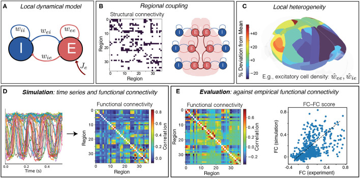
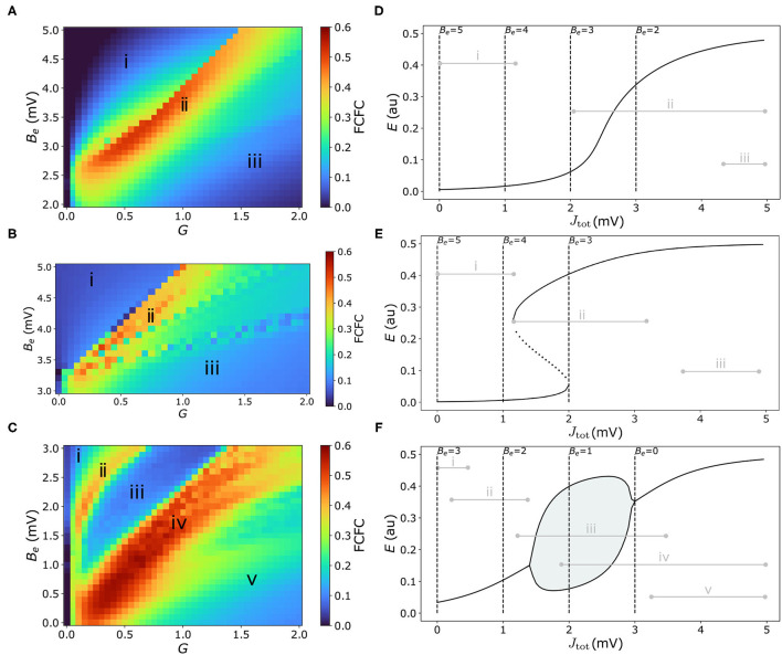
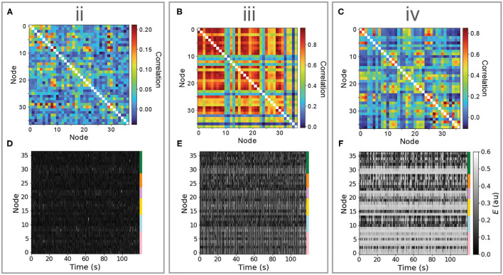
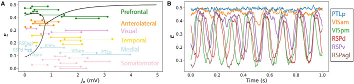
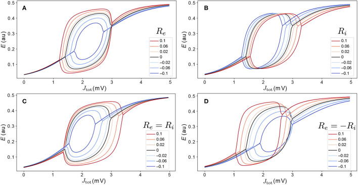
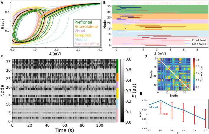
New brain atlases with high spatial resolution and whole-brain coverage have rapidly advanced our knowledge of the brain's neural architecture, including the systematic variation of excitatory and inhibitory cell densities across the mammalian cortex. But understanding how the brain's microscale physiology shapes brain dynamics at the macroscale has remained a challenge. While physiologically based mathematical models of brain dynamics are well placed to bridge this explanatory gap, their complexity can form a barrier to providing clear mechanistic interpretation of the dynamics they generate. In this work, we develop a neural-mass model of the mouse cortex and show how bifurcation diagrams, which capture local dynamical responses to inputs and their variation across brain regions, can be used to understand the resulting whole-brain dynamics. We show that strong fits to resting-state functional magnetic resonance imaging (fMRI) data can be found in surprisingly simple dynamical regimes-including where all brain regions are confined to a stable fixed point-in which regions are able to respond strongly to variations in their inputs, consistent with direct structural connections providing a strong constraint on functional connectivity in the anesthetized mouse. We also use bifurcation diagrams to show how perturbations to local excitatory and inhibitory coupling strengths across the cortex, constrained by cell-density data, provide spatially dependent constraints on resulting cortical activity, and support a greater diversity of coincident dynamical regimes. Our work illustrates methods for visualizing and interpreting model performance in terms of underlying dynamical mechanisms, an approach that is crucial for building explanatory and physiologically grounded models of the dynamical principles that underpin large-scale brain activity.

Keywords: brain dynamics; cell densities; dynamical systems; mouse cortex; neural mass model.

Figure 1

Simulating and evaluating a coupled neural-mass model of mouse cortical dynamics. (A) The dynamics of individual brain regions follow the Wilson–Cowan equations (Wilson and Cowan, 1972, 1973) which govern interactions between local excitatory (E) and inhibitory (I) neural populations. (B) Regions are coupled together by connections defined by the AMBCA (Oh et al., 2014), represented as a directed adjacency matrix (connections shown black). A schematic shows how these long-range structural connections couple local cortical regions via excitatory projections (Breakspear, 2017). (C) Heterogeneity in local model parameters can be introduced as a perturbation that follows the measured variation in excitatory and inhibitory neural densities. Here the variation in excitatory cell density is plotted across the 37 mouse cortical areas as deviations relative to the mean level (green), using brainrender (Claudi et al., 2021) and data from Erö et al. (2018). (D) Model simulation yields activity time series for each brain region, from which pairwise linear correlations (functional connectivity, FC) are computed. (E) Model simulations are evaluated against empirical FC, averaged across 100 mice, as the Spearman correlation between all unique pairwise FC values, yielding an FC–FC score, ρ_FCFC.

Figure 2

Model performance is highly sensitive to the types of dynamical features available to the coupled dynamical network, with high FC–FC found near bifurcations and where external inputs have strong dynamical responses. (A–C) FC–FC score between model and data is plotted as a heat map in G–B_e space for the three model regimes considered here (see text): (A) “Fixed-point” regime, (B) “Hysteresis” regime, and (C) “Limit-cycle” regime. Corresponding J_tot–E bifurcation diagrams [cf. Equation (4)] for each regime are shown in the right-hand panels (D–F), showing stable E fixed points (solid), unstable E fixed points (dotted), and minima and maxima of limit-cycle oscillations (solid lines with shading). Dashed vertical lines represent the minimum J_tot corresponding to selected B_e values. Gray horizontal lines represent the range of J_tot values across regions and time for a sample simulation from the corresponding point in G–B_e space annotated in (A–C). Parameter values for each regime are in Supplementary Table S2.

Figure 3

Different dynamical features of the limit-cycle regime yield very different dynamics, including noisy deviations about a stable fixed point, synchronous oscillations, and a complex distributed dynamics featuring intermittent synchronization with high FC–FC. Here, we investigate simulated time series (lower row) and functional connectivity matrices (upper row) for three regions in B_e–G space annotated “ii,” “iii,” and “iv” in Figure 2. (A–C) Simulated functional connectivity matrices are plotted for “ii,” “iii,” and “iv,” respectively. (D–F) Simulated E time series are plotted as a node × time heat map (or “carpet plot” Aquino et al., 2020) for all brain regions for “ii,” “iii,” and “iv,” respectively. Colored bars label the six cortical divisions listed in Supplementary Table S1. In all plots, nodes are ordered as per Supplementary Table S1.

Figure 4

Resolving different ranges of inputs, J_e, experienced by different network nodes allows us to understand their variable dynamical behavior in a coupled network model. Here we focus on the point labeled “iv” in the Limit-Cycle regime (Figures 2C,F), B_e = 1.5 mV, G = 0.7 mVs, in which nodes differ substantially in their inputs, J_e, and hence their resulting dynamics. (A) Bifurcation diagram for E and a function of J_e (as Figure 2F), with ranges of net excitatory drive, J_e, across the model simulation annotated for each brain region (colored according to the six labeled divisions). All regions are ordered according to Supplementary Table S1, and are labeled for the six Medial regions, which are plotted in (B). (B) E time series for the six Medial regions—PTLp, VISam, VISpm, RSPd, RSPv, and RSPagl—shown for the final 1 s of the simulation.

Figure 5

Variations in excitatory and inhibitory cell density modify the dynamical regimes accessible to cortical regions. We model the effect of variations in excitatory and inhibitory cell density via perturbation parameters R_e and R_i, respectively, as defined in Equation (5). Relative to the nominal bifurcation diagram, R_e = R_i = 0 (black), we investigate variations in −0.1 ≤ R_e ≤ 0.1 and −0.1 ≤ R_i ≤ 0.1. Four types of variation were investigated: (A) R_e only (R_i = 0); (B) R_i only (R_e = 0); (C) R_e and R_i, such that R_e = R_i; and (D) R_e and R_i, such that R_e = −R_i. The legend indicates values of R_e.

Figure 6

Modeling spatial variation in local excitatory and inhibitory cell densities produces complex distributed dynamics. (A) Bifurcation diagrams are plotted for all cortical areas according to their excitatory and inhibitory cell densities. Regions are colored according to their labeled anatomical grouping and the homogeneous case (R_e = R_i = 0) is shown in black for comparison. (B) The type of equilibrium dynamics displayed by a given cortical region, limit cycle (blue) or fixed point (red), is plotted as a function of J_e−B_e for all cortical regions for the range of J_e−B_e they experience across the model simulation. Nodes are ordered as per Supplementary Table S1 and shading reflects the six anatomical groupings labeled in A. Dashed lines shown at the top correspond to the uniform case (R_e = R_i = 0) for comparison. (C) Simulated time series for all brain areas are plotted as a heat map. Colors annotated to the right label the six anatomical groupings listed in A. (D) Simulated functional connectivity matrix. (E) FC–FC score as a function of the scaling parameter, σ, Equation (6). Results are shown for the model constrained by excitatory and inhibitory cell-density data (blue) and the permutation-based null distribution shown as mean ± standard deviation (red).

References

1. Allegra Mascaro A. L., Falotico E., Petkoski S., Pasquini M., Vannucci L., Tort-Colet N., et al. . (2020). Experimental and computational study on motor control and recovery after stroke: toward a constructive loop between experimental and virtual embodied neuroscience. Front. Syst. Neurosci. 14, 31. 10.3389/fnsys.2020.00031 - DOI - PMC - PubMed
1. Aquino K. M., Fulcher B., Oldham S., Parkes L., Gollo L., Deco G., et al. . (2021). On the intersection between data quality and dynamical modelling of large-scale fMRI signals. NeuroImage. 119051. 10.1016/j.neuroimage.2022.119051 - DOI - PubMed
1. Aquino K. M., Fulcher B. D., Parkes L., Sabaroedin K., Fornito A. (2020). Identifying and removing widespread signal deflections from fMRI data: Rethinking the global signal regression problem. NeuroImage 212, 116614. 10.1016/j.neuroimage.2020.116614 - DOI - PubMed
1. Aquino K. M., Robinson P. A., Schira M. M., Breakspear M. J. (2014). Deconvolution of neural dynamics from fMRI data using a spatiotemporal hemodynamic response function. NeuroImage 94, 203–215. 10.1016/j.neuroimage.2014.03.001 - DOI - PubMed
1. Borisyuk R. M., Kirillov A. B. (1992). Bifurcation analysis of a neural network model. Biol. Cybern. 66, 319–325. - PubMed