

Directional Preference in Avian Midbrain Saliency Computing Nucleus Reflects a Well-Designed Receptive Field Structure
- PMID: 35565569
- PMCID: PMC9105111
- DOI: 10.3390/ani12091143
Directional Preference in Avian Midbrain Saliency Computing Nucleus Reflects a Well-Designed Receptive Field Structure
Abstract
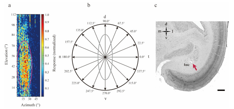
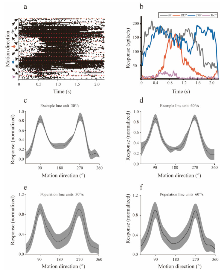
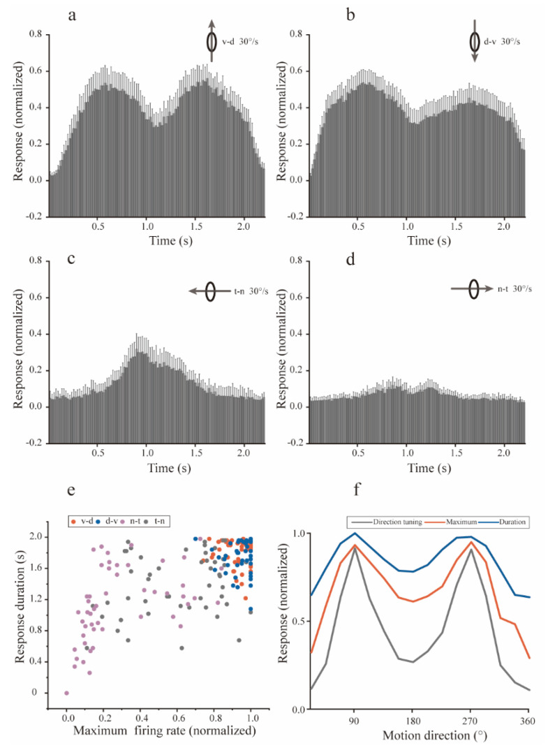
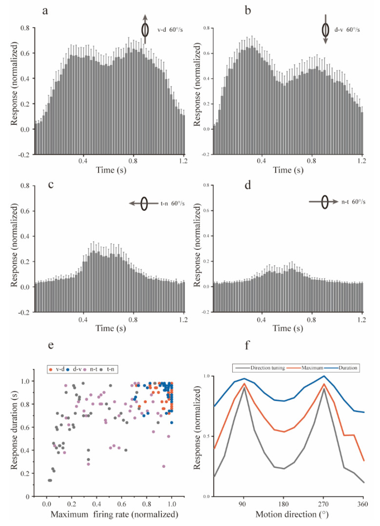
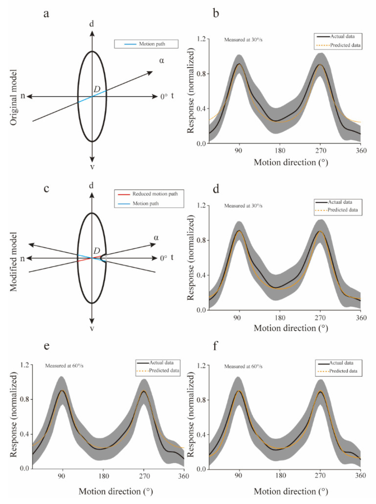
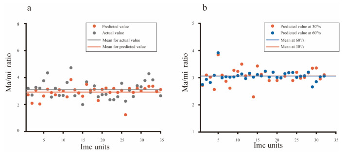
Neurons responding sensitively to motions in several rather than all directions have been identified in many sensory systems. Although this directional preference has been demonstrated by previous studies to exist in the isthmi pars magnocellularis (Imc) of pigeon (Columba livia), which plays a key role in the midbrain saliency computing network, the dynamic response characteristics and the physiological basis underlying this phenomenon are unclear. Herein, dots moving in 16 directions and a biologically plausible computational model were used. We found that pigeon Imc's significant responses for objects moving in preferred directions benefit the long response duration and high instantaneous firing rate. Furthermore, the receptive field structures predicted by a computational model, which captures the actual directional tuning curves, agree with the real data collected from population Imc units. These results suggested that directional preference in Imc may be internally prebuilt by elongating the vertical axis of the receptive field, making predators attack from the dorsal-ventral direction and conspecifics flying away in the ventral-dorsal direction, more salient for avians, which is of great ecological and physiological significance for survival.
Keywords: biological plausibility; computational model; isthmi pars magnocellularis; motion direction; pigeon.
Conflict of interest statement
The authors declare no conflict of interest.
Figures
Similar articles
-
Superimposed Inhibitory Surrounds Underlying Saliency-Based Stimulus Selection in Avian Midbrain Isthmi Pars Magnocellularis.Integr Zool. 2025 Feb 10. doi: 10.1111/1749-4877.12957. Online ahead of print. Integr Zool. 2025. PMID: 39929719
-
Detection of a temporal salient object benefits from visual stimulus-specific adaptation in avian midbrain inhibitory nucleus.Integr Zool. 2024 Mar;19(2):288-306. doi: 10.1111/1749-4877.12715. Epub 2023 Apr 12. Integr Zool. 2024. PMID: 36893724
-
Spatial Dependence of Stimulus Competition in the Avian Nucleus Isthmi Pars Magnocellularis.Brain Behav Evol. 2019;93(2-3):137-151. doi: 10.1159/000500192. Epub 2019 Aug 15. Brain Behav Evol. 2019. PMID: 31416080 Free PMC article.
-
The efferent projections of the dorsal and ventral pallidal parts of the pigeon basal ganglia, studied with biotinylated dextran amine.Neuroscience. 1997 Dec;81(3):773-802. doi: 10.1016/s0306-4522(97)00204-2. Neuroscience. 1997. PMID: 9316028 Review.
-
Assessment of the capacity of human subjects and S-I neurons to distinguish opposing directions of stimulus motion across the skin.Brain Res. 1985 Dec;357(3):187-212. doi: 10.1016/0165-0173(85)90024-4. Brain Res. 1985. PMID: 3913492 Review.
Cited by
-
Synaptic properties of mouse tecto-parabigeminal pathways.Front Syst Neurosci. 2023 May 12;17:1181052. doi: 10.3389/fnsys.2023.1181052. eCollection 2023. Front Syst Neurosci. 2023. PMID: 37251004 Free PMC article.
-
The dynamics of stimulus selection in the nucleus isthmi pars magnocellularis of avian midbrain network.Sci Rep. 2025 May 25;15(1):18260. doi: 10.1038/s41598-025-02255-w. Sci Rep. 2025. PMID: 40414967 Free PMC article.
References
-
- Samia D., Blumstein D., Díaz M., Grim T., Ibáñez-Álamo J., Jokimäki J., Tätte K., Markó G., Tryjanowski P., Moller A. Rural-Urban Differences in Escape Behavior of European Birds across a Latitudinal Gradient. Front. Ecol. Evol. 2017;5:66. doi: 10.3389/fevo.2017.00066. - DOI
-
- Carlen E., Li R., Winchell K. Urbanization predicts flight initiation distance in feral pigeons (Columba livia) across New York City. Anim. Behav. 2021;178:229–245. doi: 10.1016/j.anbehav.2021.06.021. - DOI
-
- Morelli F., Benedetti Y., Díaz M., Grim T., Ibáñez-Álamo J., Jokimäki J., Kaisanlahti-Jokimäki M.-L., Tätte K., Markó G., Jiang Y., et al. Contagious fear: Escape behavior increases with flock size in European gregarious birds. Ecol. Evol. 2019;9:6096–6104. doi: 10.1002/ece3.5193. - DOI - PMC - PubMed
-
- Knudsen E.I., Schwarz J.S. The Optic Tectum: A Structure Evolved for Stimulus Selection. Evol. Nerv. Syst. 2017;1:387–408. doi: 10.1016/b978-0-12-804042-3.00016-6. - DOI
-
- Blumstein D. What chasing birds can teach us about predation risk effects: Past insights and future directions. J. Ornithol. 2019;160:587–592. doi: 10.1007/s10336-019-01634-1. - DOI
LinkOut - more resources
Full Text Sources
Miscellaneous
