Quantification of vascular networks in photoacoustic mesoscopy

Abstract

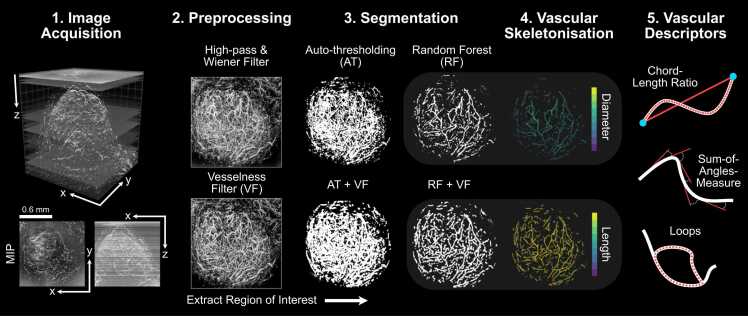
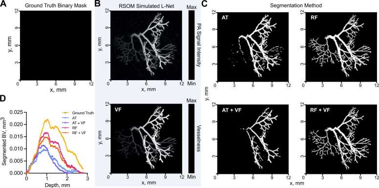
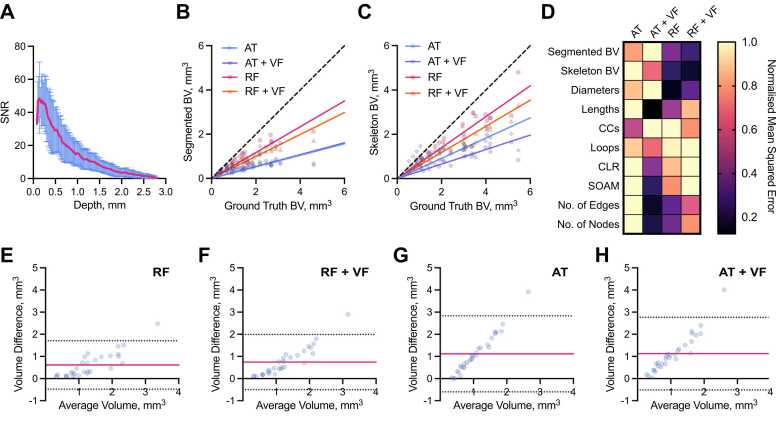
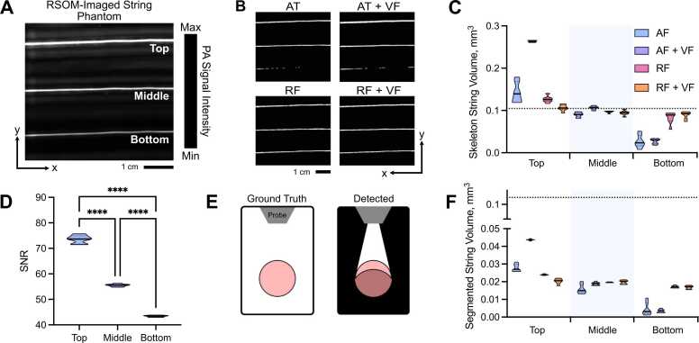
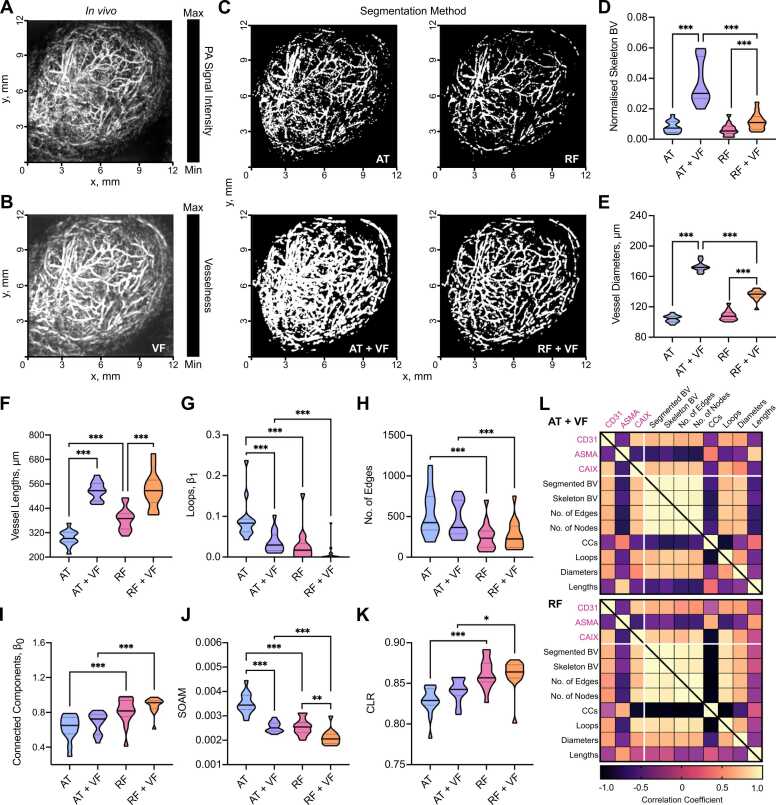
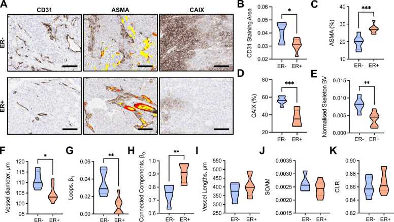
Mesoscopic photoacoustic imaging (PAI) enables non-invasive visualisation of tumour vasculature. The visual or semi-quantitative 2D measurements typically applied to mesoscopic PAI data fail to capture the 3D vessel network complexity and lack robust ground truths for assessment of accuracy. Here, we developed a pipeline for quantifying 3D vascular networks captured using mesoscopic PAI and tested the preservation of blood volume and network structure with topological data analysis. Ground truth data of in silico synthetic vasculatures and a string phantom indicated that learning-based segmentation best preserves vessel diameter and blood volume at depth, while rule-based segmentation with vesselness image filtering accurately preserved network structure in superficial vessels. Segmentation of vessels in breast cancer patient-derived xenografts (PDXs) compared favourably to ex vivo immunohistochemistry. Furthermore, our findings underscore the importance of validating segmentation methods when applying mesoscopic PAI as a tool to evaluate vascular networks in vivo.

Keywords: Photoacoustic imaging; Segmentation; Topology; Vasculature.

Fig. 1

The mesoscopic photoacoustic image analysis pipeline. 1) Images are acquired and reconstructed at a resolution of 20 × 20×4 µm³ (PDX tumour example shown with axial and lateral maximum intensity projections – MIPs). 2) Image volumes are pre-processed to remove noise and homogenise the background signal (high-pass and Wiener filtering followed by slice-wise background correction). Vesselness image filtering (VF) is an optional and additional feature enhancement method. 3) Regions of interest (ROIs) are extracted and segmentation is performed on standard and VF images using auto-thresholding (AT or AT + VF, respectively) or random forest-based segmentation with ilastik (RF or RF + VF, respectively). 4) Each segmented image volume is skeletonised (skeletons with diameter and length distributions shown for RF and RF + VF, respectively). 5) Statistical and topological analyses are performed on each skeleton to quantify vascular structures for a set of vascular descriptors. All images in steps 2–4 are shown as x-y MIPs.

Fig. 2

Exemplar vascular architectures generated in silico and processed through our photoacoustic image analysis pipeline. (A-C) XY maximum intensity projections of L-net vasculature. (A) Ground truth L-Net binary mask used to simulate raster-scanning optoacoustic mesoscopy (RSOM) image shown in (B, top) and subsequent optional vesselness filtering (VF) (B, bottom). (C) Segmented binary masks generated using either auto-thresholding (AT), auto-thresholding after vesselness filtering (AT + VF), random forest classification (RF); or random forest classification after vesselness filtering (RF+VF). (D) Segmented blood volume (BV) average across L-net image volumes, plotted against image volume depth (mm). For (D) n = 30 L-nets. See Supplementary Movie 1 for 3D visualisation.

Fig. 3

Learning-based random forest classifier outperforms rule-based auto-thresholding in segmenting simulated PAI vascular networks. (A) Depth-wise comparison of signal-to-noise ratio (SNR) measured in PAI-simulated L-nets across depth. (B,C) A comparison between ground truth blood volume (BV) and (B) segmented or (C) skeletonised blood volumes (BV). The dashed line indicates a 1:1 relationship. (D) Heat map displaying normalised (with respect to the maximum of each individual descriptor) mean-squared error comparing our vascular descriptors, calculated from segmented and skeletonised L-nets compared to ground truth L-nets, to each segmentation method. Abbreviations defined: connected components, β0 (CC), chord-to-length ratio (CLR), sum-of-angle measure (SOAM). (E-H) Bland-Altman plots comparing blood volume measurements from ground truth L-nets with that of each segmentation method: (E) RF, (F) RF+VF, (G) AT, (H) AT+VF. Pink lines indicate mean difference to ground truth, whilst dotted black lines indicate limits of agreement (LOA). For all subfigures n = 30 L-nets.

Fig. 4

Random forest classifier outperforms auto-thresholding in segmenting a string phantom. XY maximum intensity projections of string phantom imaged with RSOM show that random forest-based segmentation outmatches auto-thresholding when correcting for depth-dependent SNR. (A) Photoacoustic mesoscopy (RSOM) image shows measured string PA signal intensity with top (0.5 mm), middle (1 mm) and bottom (2 mm) strings labelled. (B) Binary masks are shown following segmentation using: (AT) auto-thresholding; (RF) Random forest classifier; (AT+VF) vesselness filtered strings with auto-thresholding; and (RF+VF) vesselness filtered strings with random-forest classifier. (C) Skeletonised string volume calculated from segmented images of 3 strings placed at increasing depths in an agar phantom. Results from all 4 segmentation pipelines are shown. All volume comparisons (top vs. middle, top vs. bottom, middle vs. bottom) where significant (p < 0.05) except middle vs. bottom for RF+VF (p = 0.42). (D) SNR decreases with increasing depth. (E) Illumination geometry: known cross-section of string outlined (left); during measurement, signal is detected from the partially illuminated section (outlined) resulting in an underestimation in string volume (right). (F) String volume calculated pixel-wise from the segmented binary mask. (C,D,F) Data represented by truncated violin plots with interquartile range (bold) and median (dotted), * ** *=p < 0.0001 (n = 7 scans). (C,F) Dotted line indicates ground truth volume 0.105 mm³. See Supplementary Movie 2 for 3D visualisation.

Fig. 5

In vivo vascular network analyses and comparisons to ex vivo immunohistochemistry in patient-derived breast tumours are dependent on segmentation method employed. XY Maximum intensity projections of breast PDX tumours imaged with RSOM: (A) original image before segmentation; (B) original image with vesselness filtering (VF) applied; (C) a panel showing segmentation with each method (AT: auto-thresholding, AT+VF: auto-thresholding with VF, RF: random forest classifier, and RF + VF: random forest with VF). (D) Skeletonised tumour blood volume (BV) from all 4 segmentation methods normalised to ROI volume. Statistical and topological data analyses were performed on skeletonised tumour vessel vascular networks for the following descriptors: (E) Vessel diameters; (F) Vessel lengths; (G) loops normalised by network volume, β1; (H) Total number of edges; (I) Connected components normalised by network volume, β0; (J) sum-of-angle measures (SOAM); and (K) chord-to-length ratios (CLR). In panels (D-K), data are represented by truncated violin plots with interquartile range (dotted) and median (bold). Pairwise comparisons of AT vs. AT+VF, AT vs. RF, RF vs. RF+VF and AT+VF vs. RF+VF calculated using a linear mixed effects model (*= p < 0.05, **=p < 0.01, ***=p < 0.001,). (L) Matrix of correlation coefficients for comparisons between IHC, BV and vascular descriptors for (top) AT+VF and (bottom) RF segmented networks. Pearson or spearman coefficients are used as appropriate, depending on data distribution. For (D) n = 14, (E-K) n = 13 due to imaging artefact in one image which will impact our vascular descriptors. For (L) comparisons involving BV n = 14, all other vascular descriptors n = 13. See Supplementary Movie 3 for 3D visualisation.

Fig. 6

ER- PDX tumours have dense and immature vascular networks which result in hypoxic tumour tissue. (A) Exemplar IHC images of CD31, ASMA and CAIX stained ER- and ER+ tumours. Scale bar= 100 µm. Brown staining indicates positive expression of marker. ASMA sections display CD31 overlay, where red indicates areas where CD31 and ASMA are colocalised (ASMA vessel coverage) and yellow indicates areas where CD31 is alone. (B) CD31 staining area quantified from CD31 IHC sections and normalised to tumour area. (C) ASMA vessel coverage of CD31 + vessels (number of red pixels/number of red+yellow pixels, expressed as a percentage) on ASMA IHC sections. (D) CAIX total positive pixels as a percentage of the total tumour area pixels on CAIX IHC sections. (E-K) Statistical and topological data analyses comparing ER- and ER+ tumours. Data are represented by truncated violin plots with interquartile range (dotted black) and median (solid black). Comparisons between ER- and ER+ tumours made with unpaired t-test. * = p < 0.05, **=p < 0.01, ***=p < 0.001. For (B-E) ER- n = 6, ER+ n = 8. For (F-K) ER- n = 5, ER+ n = 8, one ER- image excluded with artefact that would impact the measured vascular descriptors.

References

1. Brown E., Brunker J., Bohndiek S.E. Photoacoustic imaging as a tool to probe the tumour microenvironment. Dis. Models Amp;Amp; Mech. 2019;12(7):dmm039636. doi: 10.1242/dmm.039636. - DOI - PMC - PubMed
1. Corliss B.A., Mathews C., Doty R., Rohde G., Peirce S.M. Methods to label, image, and analyze the complex structural architectures of microvascular networks. Microcirc. (N. Y., N. Y.: 1994) 2019;26(5) doi: 10.1111/micc.12520. - DOI - PMC - PubMed
1. Hanahan D., Weinberg R. a. Hallmarks of cancer: the next generation. Cell. 2011;144(5):646–674. doi: 10.1016/j.cell.2011.02.013. - DOI - PubMed
1. Krishna Priya S., Nagare R.P., Sneha V.S., Sidhanth C., Bindhya S., Manasa P., Ganesan T.S. Tumour angiogenesis—Origin of blood vessels. Int. J. Cancer. 2016;139(4):729–735. doi: 10.1002/ijc.30067. - DOI - PubMed
1. Nagy J.A., Dvorak H.F. Heterogeneity of the tumor vasculature: the need for new tumor blood vessel type-specific targets. Clin. Exp. Metastas. 2012;29(7):657–662. doi: 10.1007/s10585-012-9500-6. - DOI - PMC - PubMed
LinkOut - more resources