Prediction of Retinal Ganglion Cell Counts Considering Various Displacement Methods From OCT-Derived Ganglion Cell-Inner Plexiform Layer Thickness

Abstract

Purpose: To compare various displacement models using midget retinal ganglion cell to cone (mRGC:C) ratios and to determine viability of estimating RGC counts from optical coherence tomography (OCT)-derived ganglion cell-inner plexiform layer (GCIPL) measurements.

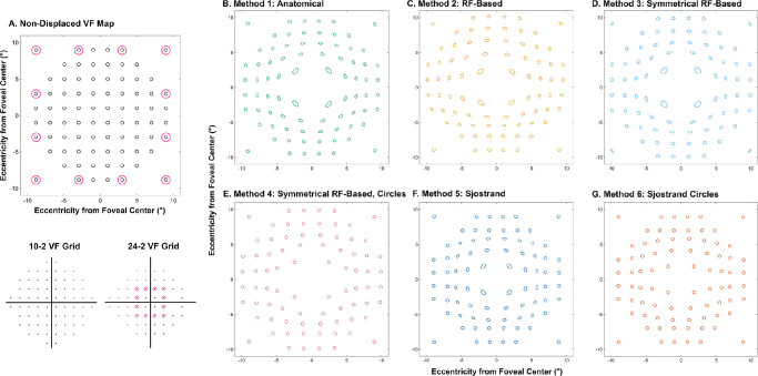
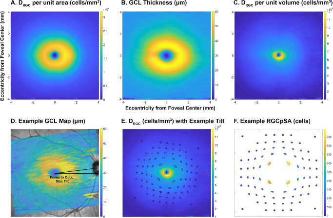
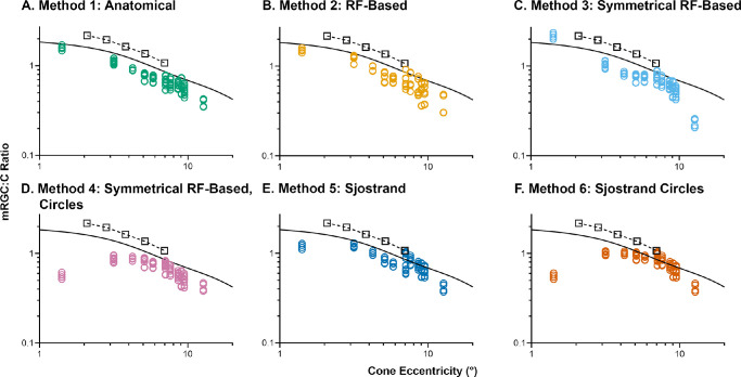
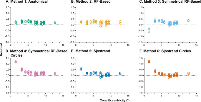
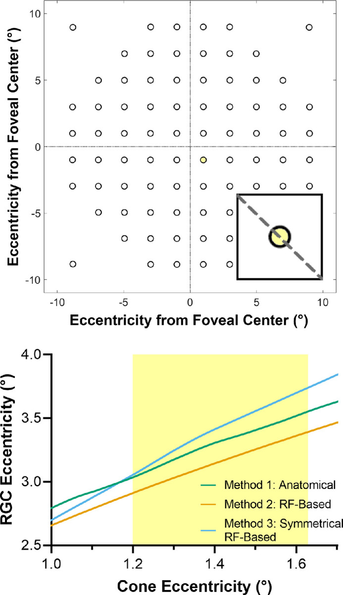
Methods: Four Drasdo model variations were applied to macular visual field (VF) stimulus locations: (1) using meridian-specific Henle fiber length along the stimulus circumference; (2) using meridian-specific differences in RGC receptive field and counts along the stimulus circumference; (3) per method (2), averaged across principal meridians; and (4) per method (3), with the stimulus center displaced only. The Sjöstrand model was applied (5) along the stimulus circumference and (6) to the stimulus center only. Eccentricity-dependent mRGC:C ratios were computed over displaced areas, with comparisons to previous models using sum of squares of the residuals (SSR) and root mean square error (RMSE). RGC counts estimated from OCT-derived ganglion cell layer (GCL) and GCIPL measurements, from 143 healthy participants, were compared using Bland-Altman analyses.

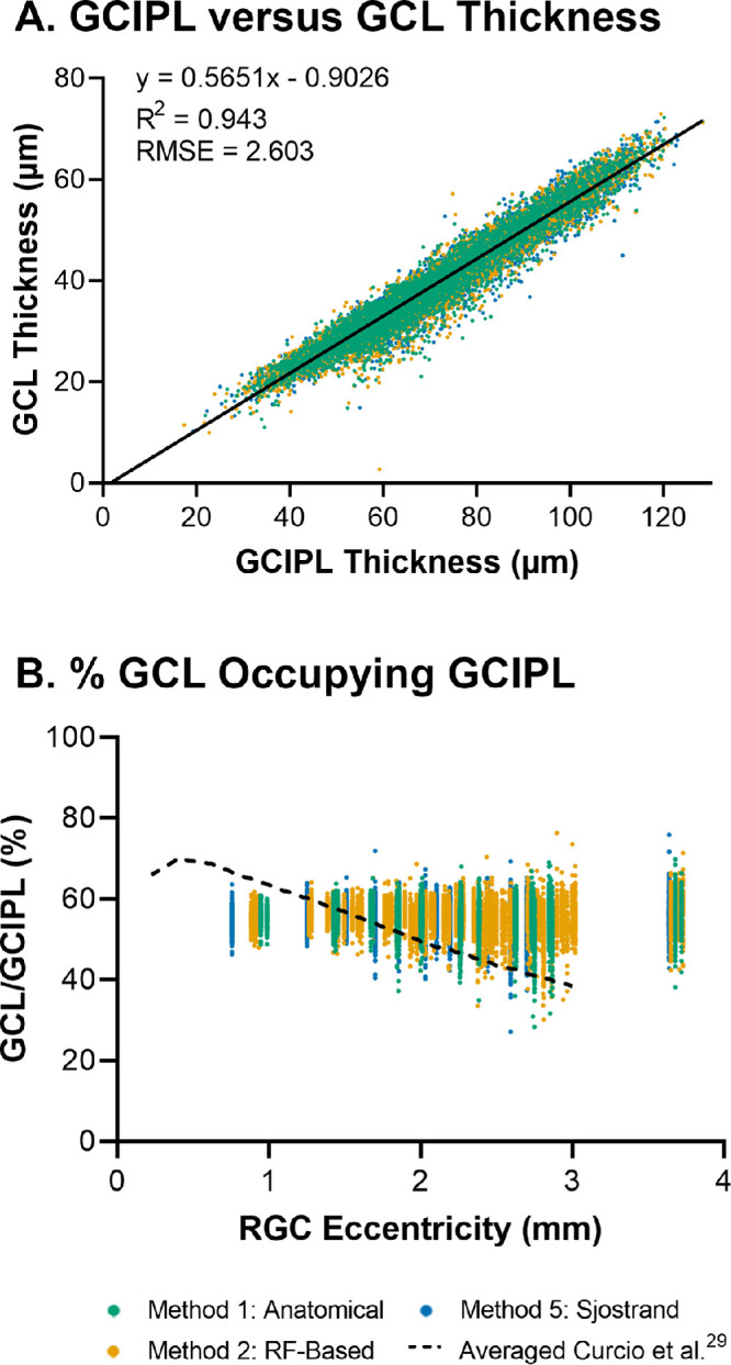
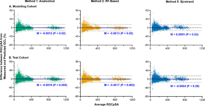
Results: Methods 1, 2, and 5 produced mRGC:C ratios most consistent with previous models (SSR 3.82, 4.07, and 3.02; RMSE 0.22, 0.23, and 0.20), while central mRGC:C ratios were overestimated by method 3 and underestimated by methods 4 and 6. RGC counts predicted from GCIPL measurements were within 16% of GCL-based counts, with no notable bias with increasing RGC counts.

Conclusions: Sjöstrand displacement and meridian-specific Drasdo displacement applied to VF stimulus circumferences produce mRGC:C ratios consistent with previous models. RGC counts can be estimated from OCT-derived GCIPL measurements.

Translational relevance: Implementing appropriate displacement methods and deriving RGC estimates from relevant OCT parameters enables calculation of the number of RGCs responding to VF stimuli from commercial instrumentation.

Figure 1.

Maps depicting the different displacement models tested in this study. All plots are displayed in VF view and right eye format. (A) The VF map with the 10-2 and paracentral 24-2 test locations prior to displacement. (B) Method 1 (anatomic) used displacement based on Henle fiber length applied along the circumference of each VF test location. (C) Method 2 (RF based) used displacement computed from the difference between cumulative RGC RF and RGC body counts, applied along the circumference of each VF test location. (D) Method 3 (symmetrical RF based) used a similar principle to method 2, except with a single displacement curve utilized regardless of angular location. (E) Method 4 (symmetrical RF based, circles) used the same displacement curve as method 3, except with displacement of the VF test location center only. (F) Method 5 (Sjöstrand) applied displacement per the Sjöstrand model along the circumference of each VF location. (G) Method 6 (Sjöstrand, circles) used the Sjöstrand model with displacement of the VF test location center only.

Figure 2.

Generation of RGC volumetric data for individual RGCpSA calculation. (A) Map of RGC density (D_RGC) in cells per square millimeter, interpolated from principal meridian data from Curcio and Allen. (B) GCL thickness map in micrometers, averaged across data from the modeling cohort. (C) D_RGC in cells per cubed millimeter, calculated from A and B. (D) An individual participant's GCL thickness map, with the foveal center and fovea to optic disc tilt annotated. (E) The displaced VF map per method 1 (Fig. 1B) superimposed on C, rotated according to fovea to optic disc tilt; D_RGC values were averaged over these areas for this fovea to optic disc tilt. The red cross indicates the optic disc center. (F) RGCpSA calculated from D and E.

Figure 3.

mRGC:C plotted as a function of cone eccentricity with the various tested implementations of the Drasdo and Sjöstrand displacement models. The averaged mRGC:C curve reported by Watson (black line) and mRGC:C ratios reported by Masri et al. (black squares and dashed line) are depicted as points of comparison. The x and y axes are in log₁₀ units for consistency with Figure 14 in Watson.

Figure 4.

Error in calculated mRGC:C per implementations of the Drasdo and Sjöstrand models relative to the Watson model, plotted as a function of cone eccentricity. The y axis units are per Figure 3.

Figure 5.

(A) Linear regression model describing the relationship between GCIPL thickness and GCL thickness in the modeling cohort. GCIPL and GCL thicknesses were averaged over displaced VF locations per methods 1, 2, and 5 (Fig. 1). Coefficient of determination (R²) and RMSE for the shared linear regression model across all methods are also shown. (B) The percentage of the GCL occupying the GCIPL as a function of RGC eccentricity in the modeling cohort. Data averaged across temporal and nasal meridians from Curcio et al. are included for reference.

Figure 6.

Bland–Altman comparisons between RGCpSA calculated from predicted versus measured GCL thicknesses for the modeling and test cohorts and for methods 1, 2, and 5, with predicted GCL thicknesses from GCIPL measurements as per Figure 4. Black dashed and dotted lines indicate the biases and 95% limits of agreement, respectively. The dark blue solid lines indicate the linear regression models through the data with corresponding slope values (M).

Figure 7.

Differences in calculated displacement for different implementations of the Drasdo model along the –45 degree meridian (gray dashed line) for the inferonasal central VF test location (yellow shading). The gradient of the displacement curve across the VF test location for method 3 appears steeper than for methods 1 and 2, resulting in a larger ellipse area along this axis and contributing to greater C_RGC for method 3.