Meta-matching as a simple framework to translate phenotypic predictive models from big to small data

Abstract

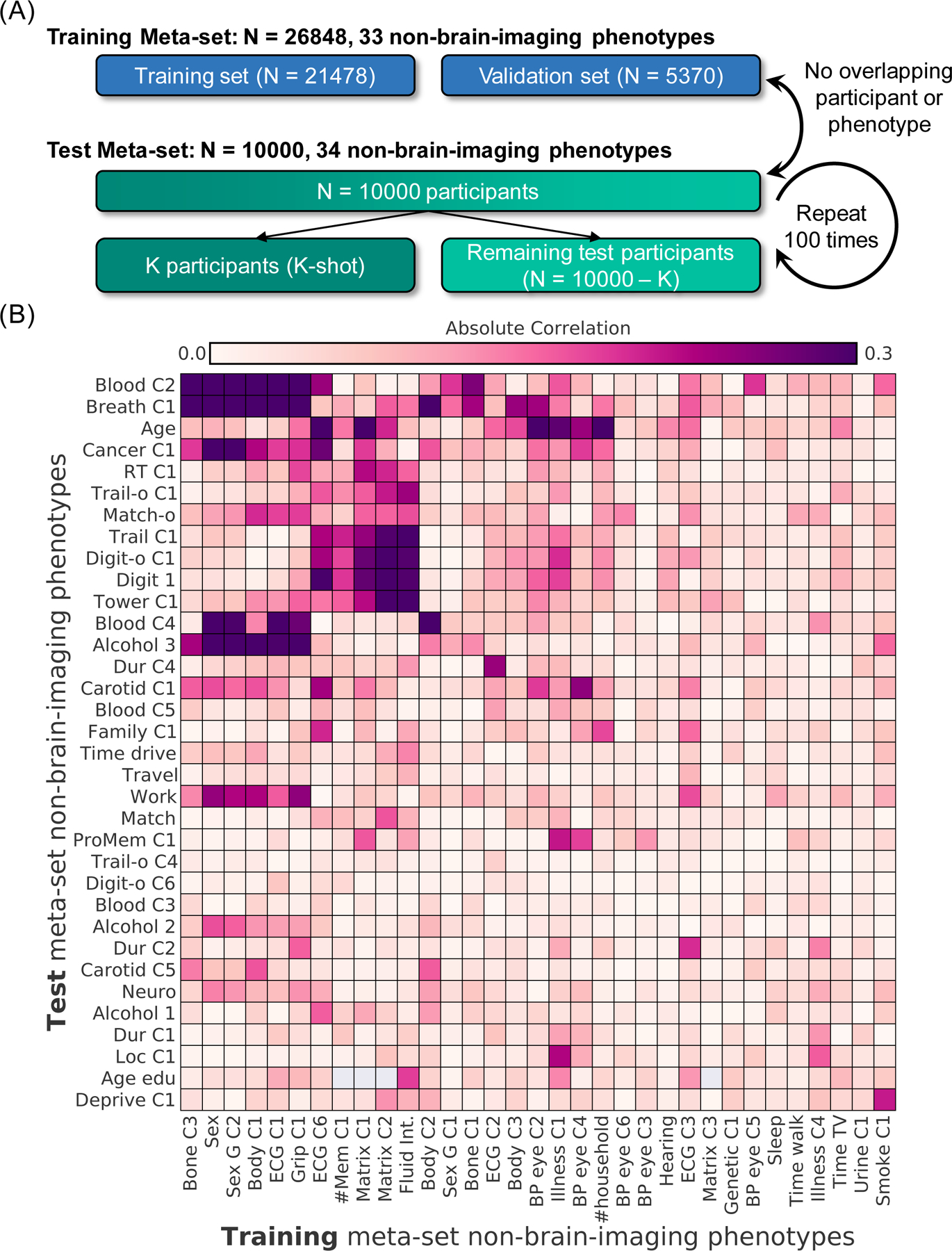
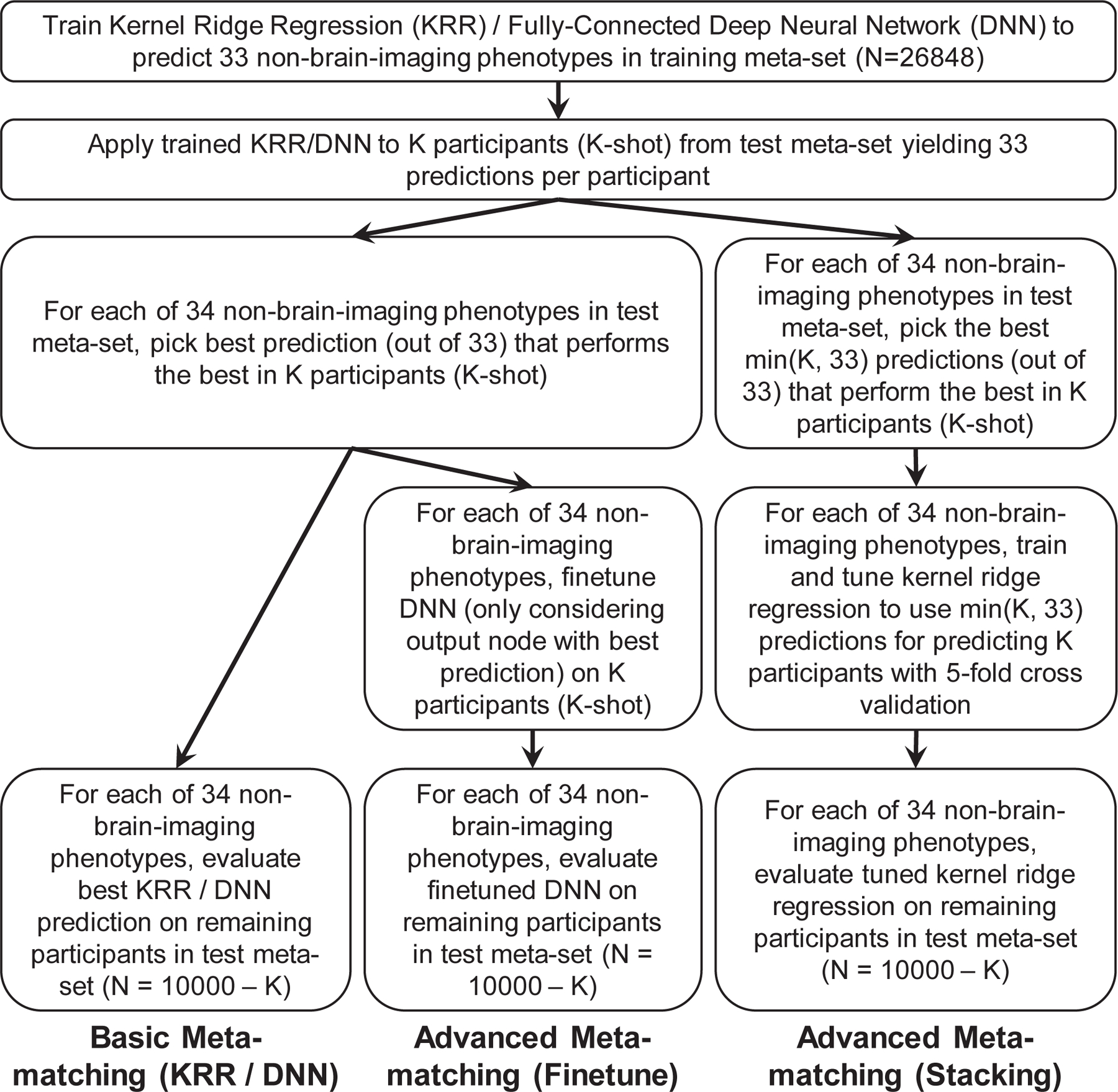
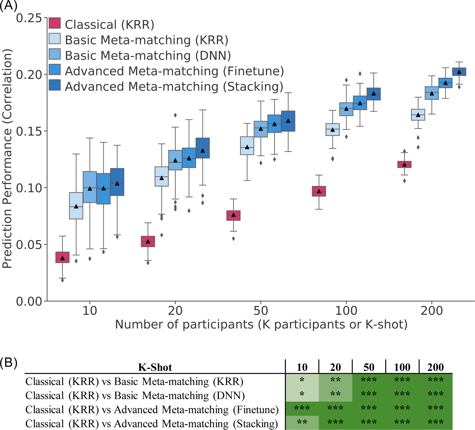
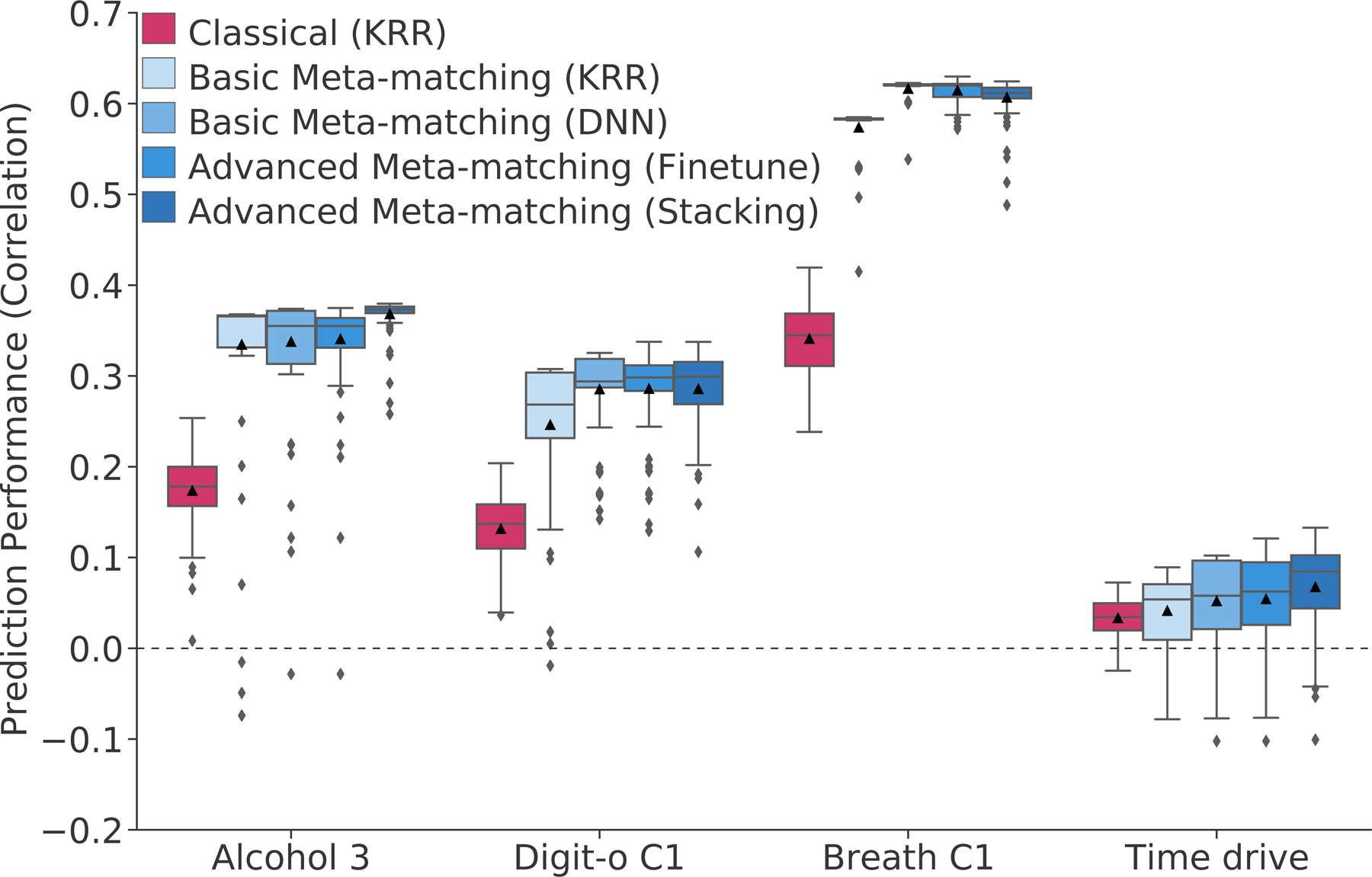
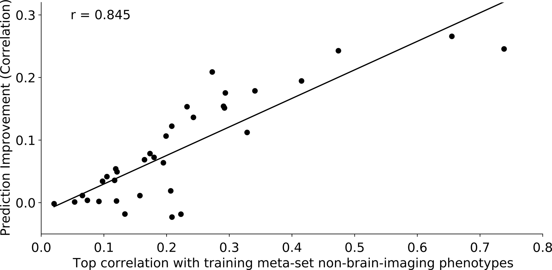
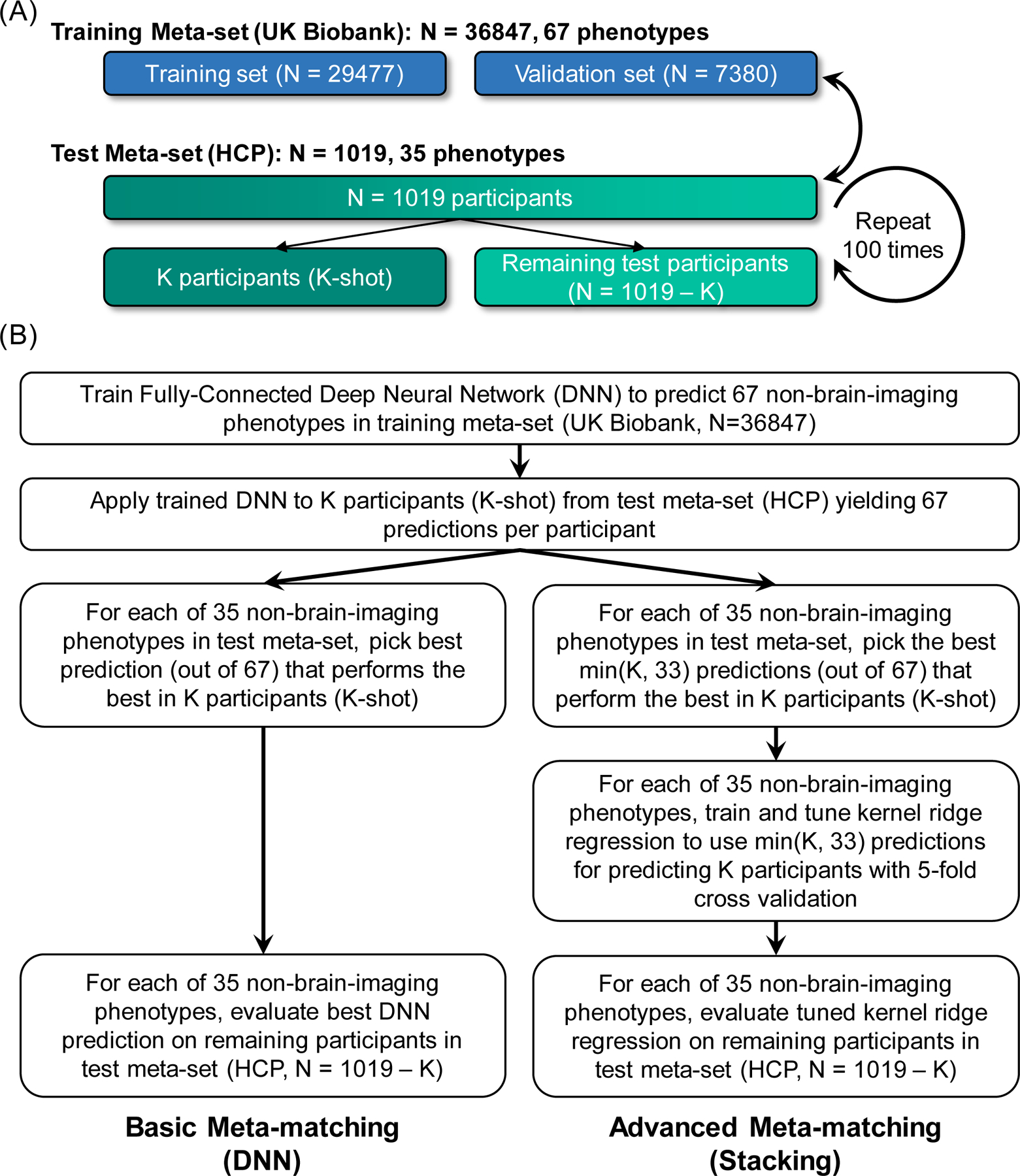
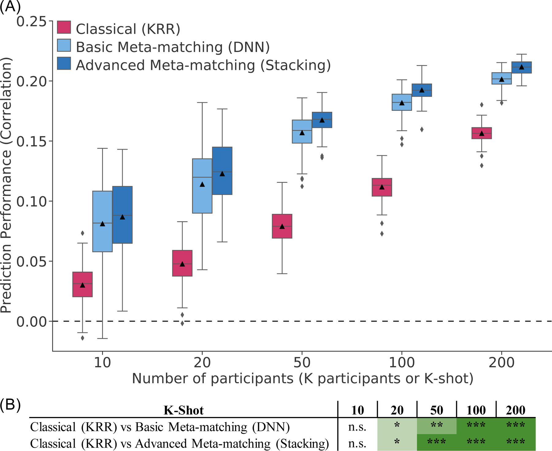
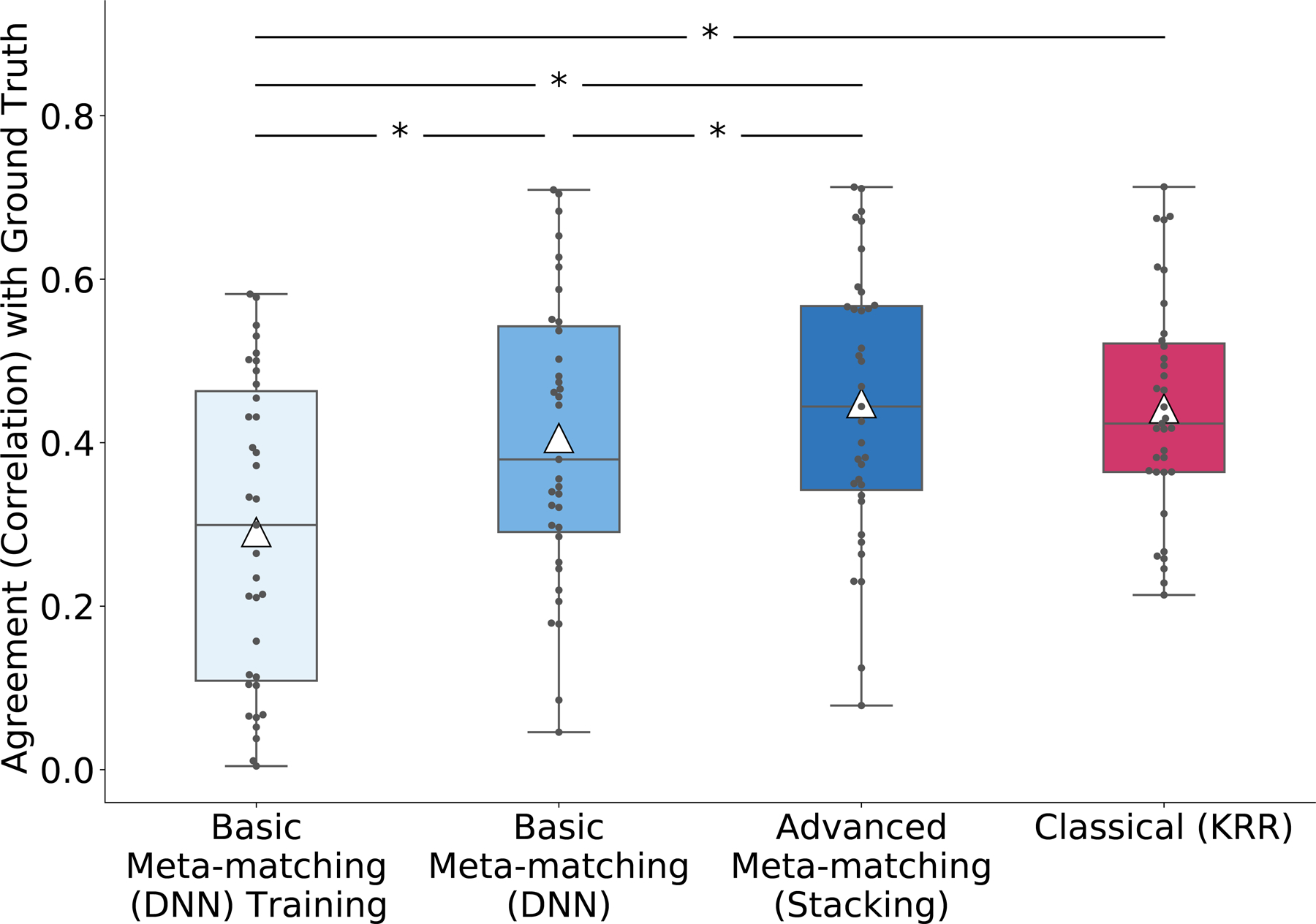
We propose a simple framework-meta-matching-to translate predictive models from large-scale datasets to new unseen non-brain-imaging phenotypes in small-scale studies. The key consideration is that a unique phenotype from a boutique study likely correlates with (but is not the same as) related phenotypes in some large-scale dataset. Meta-matching exploits these correlations to boost prediction in the boutique study. We apply meta-matching to predict non-brain-imaging phenotypes from resting-state functional connectivity. Using the UK Biobank (N = 36,848) and Human Connectome Project (HCP) (N = 1,019) datasets, we demonstrate that meta-matching can greatly boost the prediction of new phenotypes in small independent datasets in many scenarios. For example, translating a UK Biobank model to 100 HCP participants yields an eight-fold improvement in variance explained with an average absolute gain of 4.0% (minimum = -0.2%, maximum = 16.0%) across 35 phenotypes. With a growing number of large-scale datasets collecting increasingly diverse phenotypes, our results represent a lower bound on the potential of meta-matching.

Figure 1.. Experimental setup for meta-matching in the UK Biobank.

The goal of meta-matching is to translate predictive models from big datasets to new unseen phenotypes in independent small datasets. (A) The UK Biobank dataset (Jan 2020 release) was divided into a training meta-set comprising 26,848 participants and 33 phenotypes, and a test meta-set comprising independent 10,000 participants and 34 other phenotypes. It is important to emphasize that no participant or phenotype overlapped between training and test meta-sets. The test meta-set was in turn split into K participants (K = 10, 20, 50, 100, 200) and remaining 10,000-K participants. The group of K participants mimicked studies with traditionally common sample sizes. This split was repeated 100 times for robustness. (B) Absolute Pearson’s correlations between phenotypes in training and test metasets. Each row represents one test meta-set phenotype. Each column represents one training meta-set phenotype. Figures S2 and S3 show correlation plots for phenotypes within training and test meta-sets. Dictionary of phenotypes is found in Tables S1 and S2.

Figure 2.. Application of basic and advanced meta-matching to the UK Biobank.

The meta-matching framework can be instantiated using different machine learning algorithms. Here, we incorporated kernel ridge regression (KRR) and fully-connected feedforward deep neural network (DNN) within the meta-matching framework. We proposed two classes of meta-matching algorithms: basic and advanced. In the case of basic meta-matching, we considered two variants: basic meta-matching (KRR) and basic meta-matching (DNN). In the case of advanced meta-matching, we considered two variants: advanced meta-matching (finetune) and advanced meta-matching (stacking). Both advanced meta-matching variants utilized the DNN. See text for more details.

Figure 3.. Meta-matching reliably outperforms predictions from classical kernel ridge regression (KRR) in the UK Biobank.

(A) Prediction performance (Pearson’s correlation) averaged across 34 phenotypes in the test meta-set (N = 10,000 – K). The K participants were used to train and tune the models (Figure 2). Boxplots represent variability across 100 random repeats of K participants (Figure 1A). Whiskers represent 1.5 inter-quartile range. (B) Statistical difference between the prediction performance (Pearson’s correlation) of classical (KRR) baseline and meta-matching algorithms. P values were calculated based on a two-sided bootstrapping procedure (see Methods). “*” indicates p < 0.05 and statistical significance after multiple comparisons correction (FDR q < 0.05). “**” indicates p < 0.001 and statistical significance after multiple comparisons correction (FDR q < 0.05). “***” indicates p < 0.00001 and statistical significance after multiple comparisons correction (FDR q < 0.05). “n.s.” indicates no statistical significance (p ≥ 0.05) or did not survive FDR correction. Green color indicates that meta-matching methods were statistically better than classical (KRR). The actual p values and statistical comparisons among all algorithms are found in Figure S4. Prediction performance measured using coefficient of determination (COD) is found in Figure S5.

Figure 4.. Examples of phenotypic prediction performance in the test meta-set (N = 9,900) in the case of 100-shot learning.

Here, prediction performance was measured using Pearson’s correlation. “Alcohol 3” (average weekly beer plus cider intake) was most frequently matched to “Bone C3” (bone-densitometry of heel principal component 3). “Digit-o C1” (symbol digit substitution online principal component 1) was most frequently matched to “Matrix C1” (matrix pattern completion principal component 1). “Breath C1” (spirometry principal component 1) was most frequently matched to “Grip C1” (hand grip strength principal component 1). “Time drive” (Time spent driving per day) was most frequently matched to “BP eye C3” (blood pressure & eye measures principal component 3). For each boxplot, the horizontal line indicates the median and the black triangle indicates the mean. The bottom and top edges of the box indicate the 25th and 75th percentiles respectively. Whiskers correspond to 1.5 times the interquartile range. Outliers are defined as data points beyond 1.5 times the interquartile range. Figure S7 shows an equivalent figure using coefficient of determination (COD) as the prediction performance measure.

Figure 5.. Prediction improvements were driven by correlations between training and test meta-set phenotypes.

Vertical axis shows the prediction improvement of advanced meta-matching (stacking) with respect to classical (KRR) baseline under the 100-shot scenario. Prediction performance was measured using Pearson’s correlation. Each dot represents a test meta-set phenotype. Horizontal axis shows each test phenotype’s top absolute Pearson’s correlation with phenotypes in the training meta-set. Test phenotypes with stronger correlations with at least one training phenotype led to greater prediction improvement with meta-matching. Similar conclusions were obtained with coefficient of determination (Figure S8).

Figure 6.. Experiment setup for meta-matching in the Human Connectome Project (HCP).

(A) The training meta-set comprised 36,847 UK Biobank participants and 67 phenotypes. The test meta-set comprised 1,019 HCP participants and 36 phenotypes. It is important to emphasize that no participant or phenotype overlapped between training and test meta-sets. The test meta-set was in turn split into K participants (K = 10, 20, 50, 100, 200) and remaining 1,019-K participants. This split was repeated 100 times for robustness. (B) Application of basic and advanced meta-matching to the HCP dataset. Here, we considered basic meta-matching (DNN) and advanced meta-matching (stacking).

Figure 7.. Meta-matching reliably outperforms classical kernel ridge regression (KRR) in the HCP.

(A) Prediction performance (Pearson’s correlation) averaged across 35 phenotypes in the test meta-set (N = 1,019 – K). The K participants were used to train and tune the models (Figure 6B). Boxplots represent variability across 100 random repeats of K participants (Figure 6A). For each boxplot, the horizontal line indicates the median and the black triangle indicates the mean. The bottom and top edges of the box indicate the 25th and 75th percentiles respectively. Whiskers correspond to 1.5 times the interquartile range. Outliers are defined as data points beyond 1.5 times the interquartile range. (B) Statistical difference between the prediction performance (Pearson’s correlation) of classical (KRR) baseline and meta-matching algorithms. P values were calculated based on a two-sided bootstrapping procedure (see Methods). “*” indicates p < 0.05 and statistical significance after multiple comparisons correction (FDR q < 0.05). “**” indicates p < 0.001 and statistical significance after multiple comparisons correction (FDR q < 0.05). “***” indicates p < 0.00001 and statistical significance after multiple comparisons correction (FDR q < 0.05). “n.s.” indicates no statistical significance (p ≥ 0.05) or did not survive FDR correction. The actual p values and statistical comparisons among all algorithms are found in Figure S12. Prediction performance measured using coefficient of determination (COD) is found in Figure S13. Green color indicates that meta-matching methods were statistically better than classical (KRR).

Figure 8.. Agreement (correlation) of predictive network features with pseudo ground truth in the HCP dataset.

For both meta-matching (stacking) and classical (KRR), the Haufe transform was utilized to estimate predictive network features (PNFs) in the 100-shot scenario (N = 100). Pseudo ground truth PNFs were generated by applying the Haufe transform to a KRR model trained from the full HCP dataset (N = 1,019). PNFs was also estimated for basic meta-matching (DNN) training based on the UK Biobank (N = 29,477). We found that the PNFs derived from meta-matching (stacking) and classical (KRR) achieved similar agreement with pseudo ground truth. For each boxplot, the horizontal line indicates the median and the black triangle indicates the mean. The bottom and top edges of the box indicate the 25th and 75th percentiles respectively. Whiskers correspond to 1.5 times the interquartile range. Outliers are defined as data points beyond 1.5 times the interquartile range.

References

REFERENCES (MAIN TEXT)
1. Gabrieli JDE, Ghosh SS & Whitfield-Gabrieli S Prediction as a humanitarian and pragmatic contribution from human cognitive neuroscience. Neuron 85, 11–26 (2015). - PMC - PubMed
1. Woo CW, Chang LJ, Lindquist MA & Wager TD Building better biomarkers: Brain models in translational neuroimaging. Nat. Neurosci 20, 365–377 (2017). - PMC - PubMed
1. Varoquaux G & Poldrack RA Predictive models avoid excessive reductionism in cognitive neuroimaging. Curr. Opin. Neurobiol 55, 1–6 (2019). - PubMed
1. Eickhoff SB & Langner R Neuroimaging-based prediction of mental traits: Road to Utopia or Orwell? PLoS Biol 17, 1–6 (2019). - PMC - PubMed
1. Arbabshirani MR, Plis S, Sui J & Calhoun VD Single subject prediction of brain disorders in neuroimaging: Promises and pitfalls. Neuroimage 145, 137–165 (2017). - PMC - PubMed
REFERENCES (METHODS)
1. Sudlow C et al. UK Biobank: An Open Access Resource for Identifying the Causes of a Wide Range of Complex Diseases of Middle and Old Age. PLoS Med 12, 1–10 (2015). - PMC - PubMed
1. Van Essen DC et al. The WU-Minn Human Connectome Project: An overview. Neuroimage 80, 62–79 (2013). - PMC - PubMed
1. Varoquaux G et al. Assessing and tuning brain decoders: Cross-validation, caveats, and guidelines. Neuroimage 145, 166–179 (2017). - PubMed
1. Scheinost D et al. Ten simple rules for predictive modeling of individual differences in neuroimaging. Neuroimage 193, 35–45 (2019). - PMC - PubMed
1. Tan C et al. A survey on deep transfer learning. Int. Conf. Artif. neural networks 11141 LNCS, 270–279 (2018).
Publication types