Bayesian Analyses of Comparative Data with the Ornstein-Uhlenbeck Model: Potential Pitfalls

Abstract

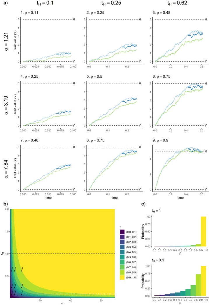
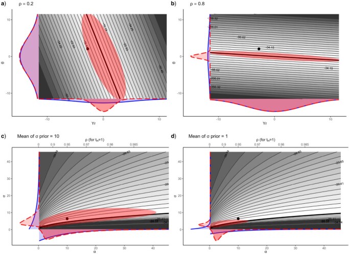
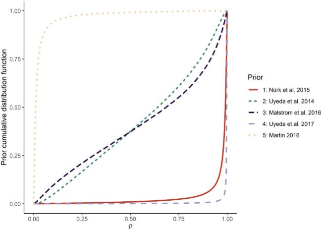
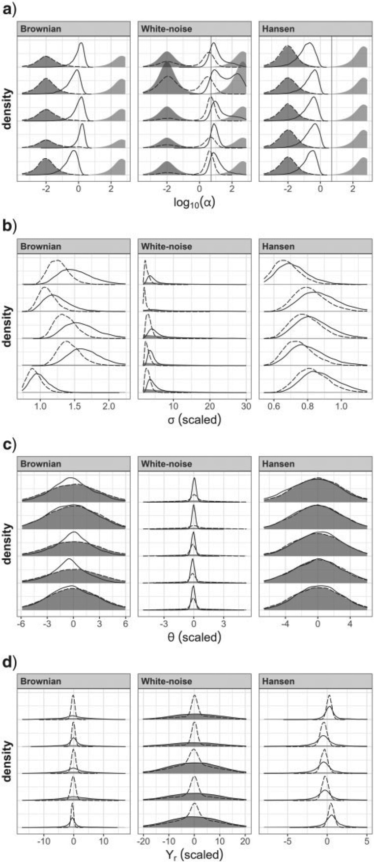
The Ornstein-Uhlenbeck (OU) model is widely used in comparative phylogenetic analyses to study the evolution of quantitative traits. It has been applied to various purposes, including the estimation of the strength of selection or ancestral traits, inferring the existence of several selective regimes, or accounting for phylogenetic correlation in regression analyses. Most programs implementing statistical inference under the OU model have resorted to maximum-likelihood (ML) inference until the recent advent of Bayesian methods. A series of issues have been noted for ML inference using the OU model, including parameter nonidentifiability. How these problems translate to a Bayesian framework has not been studied much to date and is the focus of the present article. In particular, I aim to assess the impact of the choice of priors on parameter estimates. I show that complex interactions between parameters may cause the priors for virtually all parameters to impact inference in sometimes unexpected ways, whatever the purpose of inference. I specifically draw attention to the difficulty of setting the prior for the selection strength parameter, a task to be undertaken with much caution. I particularly address investigators who do not have precise prior information, by highlighting the fact that the effect of the prior for one parameter is often only visible through its impact on the estimate of another parameter. Finally, I propose a new parameterization of the OU model that can be helpful when prior information about the parameters is not available. [Bayesian inference; Brownian motion; Ornstein-Uhlenbeck model; phenotypic evolution; phylogenetic comparative methods; prior distribution; quantitative trait evolution.].

Figure 1

a) Trait trajectories for a three-tip tree for nine different combinations of values of and . b) Value of as a function of and . The nine points correspond to the nine trajectories in (a). Note that the analysis of a given data set with a given occurs along a horizontal line of this graph. c) Priors for corresponding to a uniform prior for from 0 to 69, when or . The relative heights of the different bars match the relative distances between the isoclines in b), along the lines or (represented by dashed lines in b).

Figure 2

Example ridges in the OU likelihood. Gray shades represent the value of the log-likelihood, for a data set simulated with , of which the trait values were scaled to mean 0 and unit variance. Density plots with solid lines in the margins represent the priors. The darker areas superimposed on the likelihood surface represent the 95 highest posterior density region of the joint posterior of and (in a and b) or of and (in c and d). Density plots with dashed lines in the margins represent the marginal posteriors. The posteriors were approximated by numerical integration. Black dots represent the true values of the parameters used to simulate the data set. a) and b) represent the ridge, with fixed to its true value and with (a) or (b). In both cases, the priors for and are centered normal distributions with sd = 5. The thick black line is the top of the ridge, of equation , with the ML estimator of the mean of tip trait values (equal to 0 in this example, since trait values were scaled to 0 mean). In a), because is low, the ridge has a highly negative slope. As a consequence, the plausible range of , as constrained by the prior, corresponds to a narrow interval of high likelihood on the scale of , inducing a marginal posterior for that is narrower than its prior. In b), is high and the converse happens. c) and d) The ridge, with and fixed to their true values is represented. The prior for is in both cases an exponential distribution with mean 10. The prior for is an exponential distribution with mean 10 in c) and with mean 1 in d). The thick black line has equation , with the stationary variance of the process, set to 1 (the sample variance of the tip trait values after scaling). As grows, this line tends to be the top of the ridge. The difference with the ridge is that the top of this ridge is not completely flat. However, as one moves towards higher values, it gets ever flatter. In d), the prior for restricts inference to smaller values of than in c). As a consequence, the a priori smaller plausible values of correspond to a region around the likelihood ridge that matches smaller values. This has the effect of shifting the marginal posterior of towards smaller values. In this example, the true value of would even be excluded from the 95 credible interval, because of the prior for .

Figure 3

A set of five priors for found in the literature, translated into priors for . These priors can be observed to range from favoring a lot low values of (Martin 2016) or high values of (e.g., Uyeda et al. 2017).

Figure 4

Marginal posteriors for trees with 40 tips when fitting an OU model. Dashed curves, posteriors with the BM prior. Solid curves, posteriors with the WN prior. Shaded areas represent the priors. For , the darker and lighter areas represent the BM and WN priors, respectively, and the vertical line represents the value used in simulations. The posterior densities for five of the 20 analyses are represented (see Appendix 8 of the Supplementary material available on Dryad for graphs for all analyses). Different columns correspond to different simulation models. The rows correspond to a) , b) , c) , and d) . Note that because the analyses were carried out on scaled trait values, both the priors and the true values cannot be represented on the same graph for parameters in unit of traits (see Appendix 5 of the Supplementary material available on Dryad). The scaled version of such parameters is plotted here for comparison with priors.

Figure 5

Correlation among parameters in the joint posterior. Each plot was drawn by pooling the posterior samples of all analyses conducted on data sets that were produced with the same simulation model. a) and c) Correlation of and for inference with the OU and Hansen models, respectively. The curve is represented. b) Correlation of and for inference with the OU model. Only posterior samples with intermediate values (i.e., between 1 and 2) were included. The curve is represented. d) Correlation of and for inference with the OU model. is the average of across branches. Only posterior samples with intermediate values (i.e., between 1 and 2) were included. The curve is represented. Note that in the Hansen model, the formula of the expected relationship between and is not this curve, although in this case it comes close to it.

Figure 6

Marginal posteriors for trees with 40 tips when fitting the Hansen model with multiple selective optima. The dashed and solid curves represent the posteriors obtained with the BM and WN priors, respectively. Shaded areas represent the priors. For , the darker and lighter shaded areas represent the Brownian and WN priors, respectively. For and , the vertical line(s) represent(s) the value(s) used in simulations. The posterior densities of 5 of the 20 analyses are represented. Different columns correspond to different simulation models. The rows correspond to: a) , b) , c) the ’s (pooled together), d) , and e) (the number of selective regimes). The plots of e) are represented for for visibility, but the prior is flat from 0 to the number of branches (see Appendix 3 of the Supplementary material available on Dryad). The scaled version of parameters is plotted here for comparison with the priors, except for the ’s which have been unscaled for comparison with the true values.

Figure 7

Marginal posterior densities obtained with the reparameterized OU model. a) Posterior of , directly comparable to Figure 4a. b) Posterior of , comparable to Figure 4b, except here is unscaled for comparison with the true value. c) Posterior of . d) Posterior of (unscaled). e) Posterior of (unscaled). The data sets used here are a subset of those used for Figure 4: 5 BM () and 5 WN () data sets. The vertical lines show the true values of the parameters. The prior for was a uniform distribution. The prior for was a normal distribution centered around the sample mean of tip traits and SD of 2. Two priors were considered for , consisting of log-normal distributions with a mode at the sample variance of tip traits, and with an SD on the log scale of 0.5 (solid curves) or 2 (dashed curves). and are not parameters of the reparameterized OU model, and their values were deduced a posteriori from the values of , and (see Appendix 10 of the Supplementary material available on Dryad).

References

1. Ané C. 2008. Analysis of comparative data with hierarchical autocorrelation. Ann. Appl. Stat. 2(3):1078–1102.
1. Ané C., Ho L.S.T., Roch S.. 2017. Phase transition on the convergence rate of parameter estimation under an Ornstein-Uhlenbeck diffusion on a tree. J. Math. Biol. 74(1):355–385. - PubMed
1. Beaulieu J.M., Jhwueng D.-C., Boettiger C., O’Meara B.C.. 2012. Modeling stabilizing selection: expanding the Ornstein-Uhlenbeck model of adaptive evolution. Evolution 66(8):2369–2383. - PubMed
1. Blomberg S.P., Garland T.J., Ives A.R.. 2003. Testing for phylogenetic signal in comparative data: behavioral traits are more labile. Evolution 57(4):717–745. - PubMed
1. Boettiger C., Coop G., Ralph P. (2012). Is your phylogeny informative? Measuring the power of comparative methods. Evolution 66(7):2240–2251. - PMC - PubMed
Publication types