Influence of T-Bar on Calcium Concentration Impacting Release Probability

Abstract

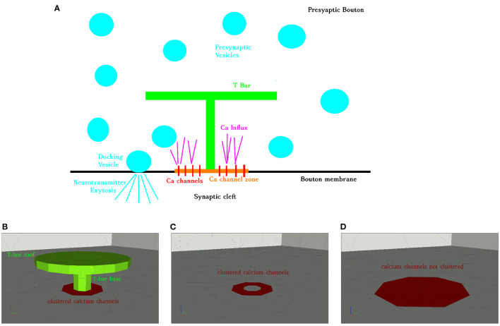
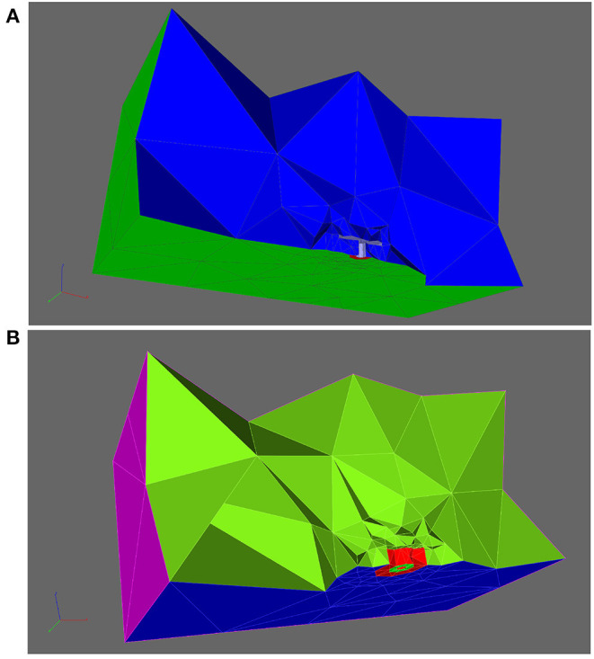
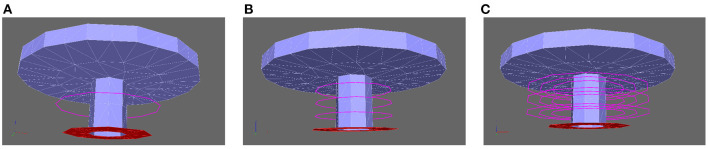
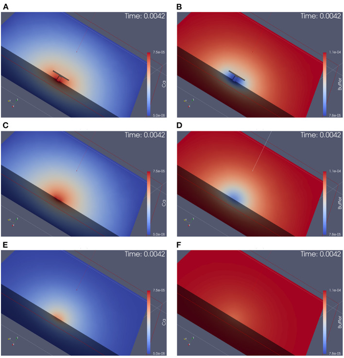
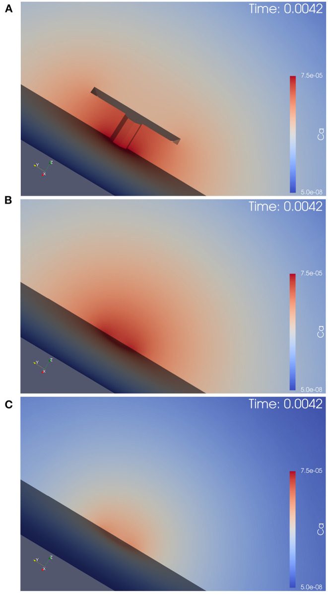
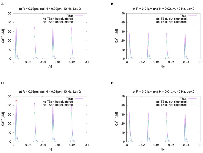
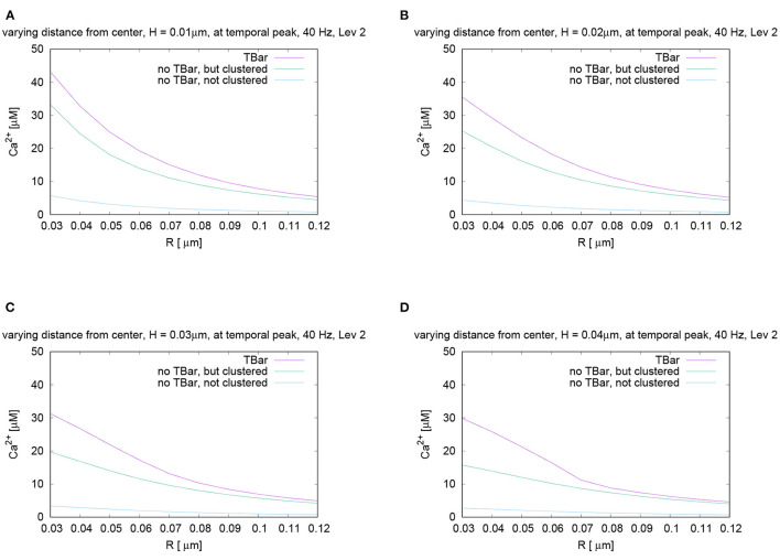
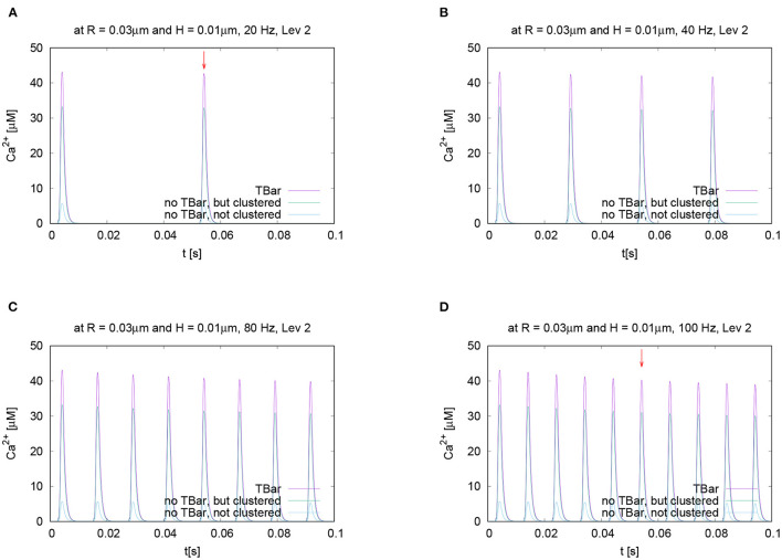
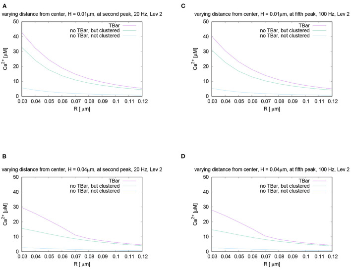
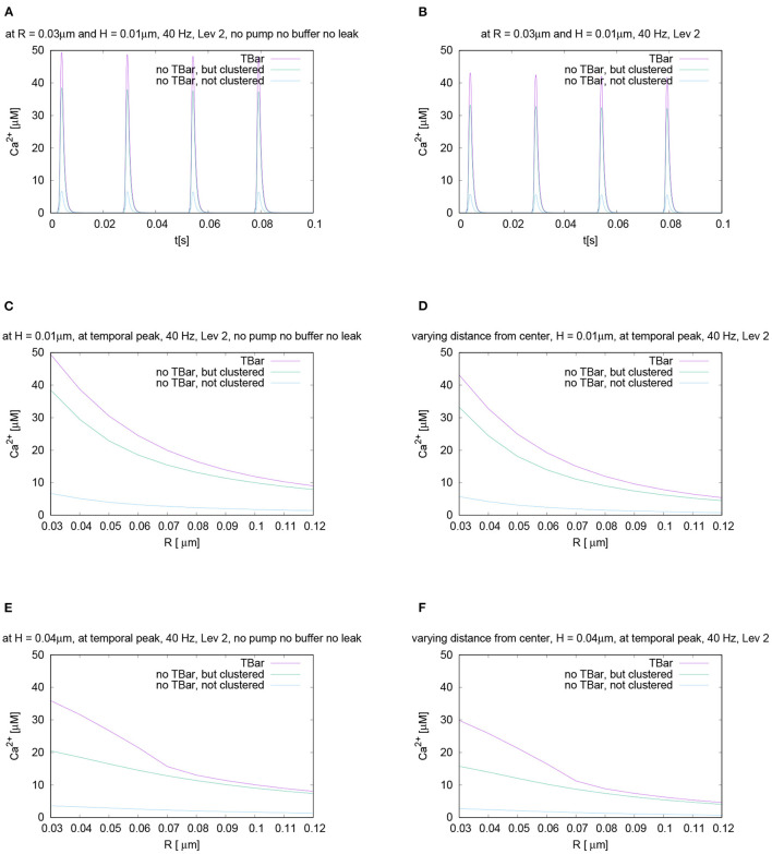
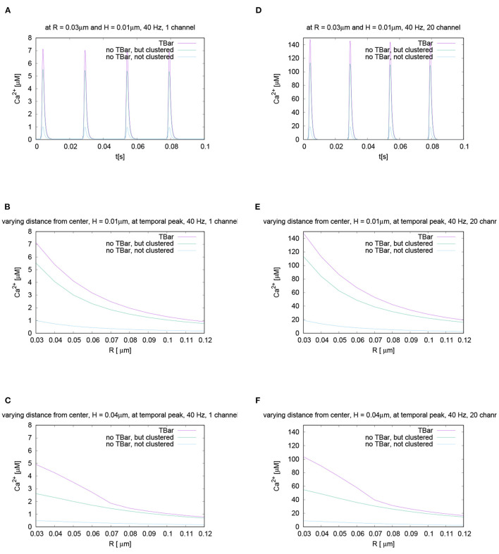
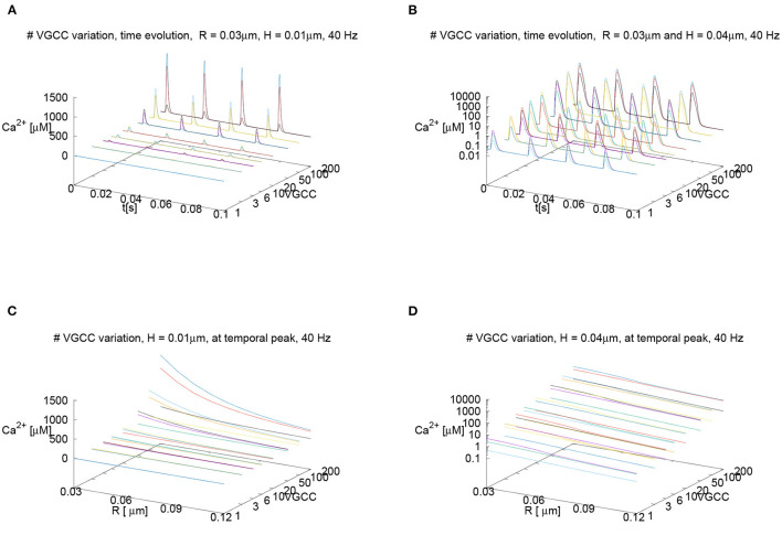
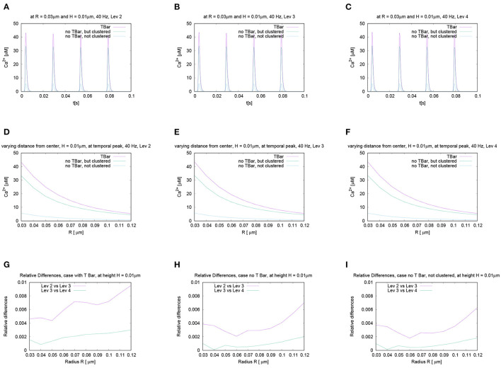
The relation of form and function, namely the impact of the synaptic anatomy on calcium dynamics in the presynaptic bouton, is a major challenge of present (computational) neuroscience at a cellular level. The Drosophila larval neuromuscular junction (NMJ) is a simple model system, which allows studying basic effects in a rather simple way. This synapse harbors several special structures. In particular, in opposite to standard vertebrate synapses, the presynaptic boutons are rather large, and they have several presynaptic zones. In these zones, different types of anatomical structures are present. Some of the zones bear a so-called T-bar, a particular anatomical structure. The geometric form of the T-bar resembles the shape of the letter "T" or a table with one leg. When an action potential arises, calcium influx is triggered. The probability of vesicle docking and neurotransmitter release is superlinearly proportional to the concentration of calcium close to the vesicular release site. It is tempting to assume that the T-bar causes some sort of calcium accumulation and hence triggers a higher release probability and thus enhances neurotransmitter exocytosis. In order to study this influence in a quantitative manner, we constructed a typical T-bar geometry and compared the calcium concentration close to the active zones (AZs). We compared the case of synapses with and without T-bars. Indeed, we found a substantial influence of the T-bar structure on the presynaptic calcium concentrations close to the AZs, indicating that this anatomical structure increases vesicle release probability. Therefore, our study reveals how the T-bar zone implies a strong relation between form and function. Our study answers the question of experimental studies (namely "Wichmann and Sigrist, Journal of neurogenetics 2010") concerning the sense of the anatomical structure of the T-bar.

Keywords: Drosophila larval NMJ; T-bar; UG4; VGCC; calcium influx; calcium microdomain; diffusion-reaction PDE model; vesicle release probability.

Figure 1

Aim of this figure: Display the biological process under consideration, and display the realization of the geometry of the anatomic structures for the three different anatomic structures under consideration. (A) Calcium influx and vesicle release at the Drosophila NMJ at an AZ with T-bar, schematic representation. (B–D): Geometric realization of typical AZs of the NMJ: We consider three basic scenarios: (A) Active zone with T-bar and clustered channels, (B) AZ without T-bar, but with clustered channels, (C) AZ without T-bar, and the channels are not clustered, but more widely distributed (the surface where the channels are located is bigger, but the channel number is assumed to be the same). Reason for the difference between (C,D): we want to probe for the influence of clustered channels in the case when no T-bar is present at the AZ. Therefore, the (red) channel zone is larger, and this reflects a biophysical change in the geometric conditions of the model. Note that the channel zones are marked with red color, and the T-bar with green color, i.e., channel zones $\mathcal{C}$ depicted with red color. Same perspective for all three cases. Scale: Diameter “table” of T-bar: 140 nm. Height of the leg: 40 nm, diameter of the leg: 30 nm. The thickness of the “table desk”: 10 nm. Diameter of the clustered channels: 70 nm, in case of not clustered channels: 140 nm.

Figure 2

Aim of this figure: Display the computational domain in order to explain the geometric Finite Element mesh basis of the simulation. Computational domain displayed opened by a cut plane to allow insight into the region where the T-bar AZ is located, and to explain the subdomains which are important to understand the regions where computations are evaluated in this study. (A): Cut of the volume mesh in case of the T-bar geometry, T-bar space left empty to account for the obstacle of the T-bar. Coarse grid. Entire computations are performed with refined grid versions. The complete 3D triangular mesh forms the computational domain $\mathcal{V}$, blue. The surface zone of calcium channels, $\mathcal{C}$, is marked in red. (B): Cut plane applied to the volume mesh, where that volume “below” the “table” of the T-bar is highlighted with red color, the subdomain $\mathcal{U}$. Note that the different colors compared to (A) do not indicate a paradigm change or other subdomains, but are applied in order to highlight the domain of interest we want to highlight here. Note also that the cut plane is located more in the front in comparison to the case of (A).

Figure 3

Aim of this figure: Display the regions where the calcium concentrations will be evaluated which arise within our simulations. The regions of evaluations are circles around the T-bar “socket”. The circles are placed such that they cover the region below the T-bar “roof” in a rather dense way, as well in height computed from the membrane base, and also in distance from the T-bar “socket”. In the Results, Section 3, we evaluate the averaged concentrations of each circle, as evaluations at only single points might not be so favorable, even though we also check that our results are independent of the computational grid. Constructing circles around the T-bar socket to measure calcium at equidistant radii and heights from the T-bar socket. Note the thin magenta colored lines around the table leg, which mark the evaluation lines. Circles constructed based upon (18). (A): One circle, (B): three circles for fixed radius, but different height, (C): various circles for different heights and different radii.

Figure 4

Simulation of calcium and buffer concentration under repetitive action potential stimulation for the three different anatomical cases. Screenshots are taken at the first calcium microdomain peak. Full simulation movies are available as Supplemental Material. The simulation movies show the computational domains disclosed by means of a cut plane. Left: calcium concentration, Right: buffer concentration. From top to down: With T-bar and clustered channels, without T-bar but channels still clustered, without T-bar and no channel clustering. (A): calcium with T-bar, (B) buffer with T-bar, (C) calcium no T-bar channels clustered, (D) buffer no T-bar channels clustered, (E) calcium no T-bar channels not clustered, and (F) buffer no T-bar channels not clustered. At each action potential, calcium enters through the VGCC calcium channels, diffuses into the presynaptic zone. Due to the limited diffusion speed, calcium accumulates close to the AZ, before it reduces again when the calcium influx reduces again, as the voltage at the membrane drops down. Calcium reduction in major part is due to the diffusion process that causes the calcium to diffuse away. In minor part, calcium buffering and calcium pumps which pump calcium out of the presynaptic bouton again also reduce calcium amount. Before when the next action potential arrives, the calcium level arrives again at initial values (also buffer concentration, which also moves by means of diffusion). At the next action potential, the same process starts again. As the screenshots are taken at peak time, we see easily that in the case of the presence of the T-bar, the concentration at peak time is higher than in the case without T-bar, but still clustered channels, and we observe further that in case without T-bar and without clustered channels, calcium concentration is much smaller. Obviously, the T-bar obstacle causes calcium accumulation below the T-bar, and channel clustering also has a positive influence upon calcium microdomain accumulation.

Figure 5

This figure displays the simulation movie screenshot at peak of calcium influx in a zoomed version of the calcium concentration for the three different anatomic scenarios, i.e., it is a magnified version of Figure 4 with the focus on the AZ center, and shows only the calcium, but not the buffer concentrations. We see the computational domain disclosed by a cut plane, and the AZ is in the center. In (A), we see the case of the T-bar with clustered channels, in (B), we see the case without T-bar, but clustered channels. In (C), we see the case without T-bar and without clustered channels. The explanations given in the caption of Figure 4 can be observed here in more detail: The T-bar enhances calcium concentration substantially, while the channel clustering has an additional influence. The lack of each one of these anatomic features reduces the calcium microdomain concentration. Hence, the T-bar and the channel clustering each have a substantial impact upon the calcium microdomain shape.

Figure 6

This figure displays quantitative evaluations of the temporal dynamics of calcium concentrations at fixed spatial locations. We display the concentration value of calcium for a given height averaged over a circle with a given radius. The height and the radius are based upon the circles as described in Section 2 and displayed in Figure 3. This means we evaluate the averaged calcium values for a fixed circle. The four sub graphics shown represent the values evaluated at four different circles with noted values of radius and height. Ordering of graphs inspired by their radius and height value i.e., bigger height upper, bigger radius on the right. The radius of calcium concentration evaluation around the (imaginative in the case without T-bar) T-bar socket center at (C) radius R = 0.03μm and height H = 0.01μm, (A) R = 0.03μm and H = 0.02μm, (D) R = 0.04μm and H = 0.01μm, and (B) R = 0.04μm and H = 0.02μm. We see that in all cases, at peak time, the concentration in the case of the T-bar is substantially elevated compared to the case without T-bar, but still clustered channels. Additionally, we see that in all cases, the concentration is the smallest in the case when the channels are not clustered and no T-bar is present. Furthermore, we see that with increasing height, i.e., distance from the membrane of the AZ, the concentrations decrease in all configurations. Also, we see that with increasing radius, the concentration profiles decrease as well.

Figure 7

Spatial profiles of calcium concentrations at a fixed time for the three different anatomic cases. The evaluations of the concentrations are performed at the first peak which is marked with a red arrow in Figure 6C, i.e., for t = 0.0042s. We evaluate the concentrations for various fixed heights H and vary the radius R, and display the averaged concentrations over the circles (compare Figure 3) around the (virtual) T-bar socket. Height locations: (A) H = 0.01μm, (B) H = 0.02μm, (C) H = 0.03μm, and (D) H = 0.04μm. This means that for a given height above the membrane respectively the “root” of the T-bar “socket” (virtual in the case when T-bar is missing), we “walk” from inside to outside for fixed height, and we “jump” from circle to circle. Obviously, in all cases, the concentration is the highest when the T-bar is present, and next, it follows the case when the channels are clustered, but the T-bar is absent. The case of not clustered channels combined with no T-bar shows strongly reduced concentrations in all cases. We observe that in all cases, the concentrations drop down the farther away we go from the center. We see a major impact of the T-bar, namely for small radius and increasing height, i.e., distance from the membrane. If we compare the case of clustered channels with and without T-bar, we observe that as long as we are close to the membrane, for small height, the values differ only by about 25%. However, the more the height grows, the bigger the difference, namely close to the T-bar “socket”. Below the (virtual) T-bar “roof”, the presence of the T-bar causes the concentration to be about a factor two bigger than when the T-bar is missing. This observation indicates that below the T-bar “roof”, vesicles “sense” a much higher calcium concentration, compared to the case without T-bar, even in the case when the channels are clustered. In the case of not clustered channels (without T-bar), the concentrations are reduced even about a factor of 10 compared to the T-bar case. Therefore, this result is a strong hint that the T-bar has quantitatively a strong impact upon the calcium concentration at the AZ.

Figure 8

Temporal evolution of the concentration overtime at a fixed spatial location. Fixed height and fixed radius averaged values for different frequencies concentration evaluation around the (imaginative in the case without T-bar) T-bar socket center at radius R = 0.03μm and height H = 0.01μm. Variation of frequency, comparing high and low frequencies. We observe a very similar behavior at the peaks concerning the relation between the three geometric configurations. Peaks of (A) 20 Hz, (B) 40 Hz (known case), (C) 80 Hz, and (D) 100 Hz. stimulation. This figure demonstrates that the variation of frequency has no substantial influence upon the relation of calcium peak concentrations when comparing the three different geometric scenarios. The graphs show that not only at the first peak, but also at later peaks, the T-bar case shows the highest concentration, followed by the case without T-bar, but clustered channels, and that the case without T-bar and with not clustered channels has much less concentration.

Figure 9

Comparison for the calcium concentration under variation of radius and height at the fixed time point for different stimulation frequencies, i.e., evaluation of the spatial profile of calcium concentrations at peak time after several action potentials, for the same time point. Note the red arrows in Figures 8A,C mark the peaks for which we perform the comparisons. Comparison of the shapes of calcium concentration for the second peak of 20 Hz stimulation (A,B), and the fifth peak of 100 Hz stimulation, which temporally coincides with the second peak of 20 Hz (C,D). We display the profiles for a height close to the membrane, and another one close to the T-bar “roof”. The behavior is practically the same as for the first peak in the 40 Hz stimulation shown in Figure 7. Also here, close to the (virtual) T-bar socket and close to the membrane, the T-bar anatomy shows about 25% more calcium than the case without T-bar but clustered channels. Close to the (virtual) T-bar “roof”, the T-bar case shows about two times more calcium concentration compared to the case without T-bar but clustered channels. As well, the case without T-bar and without clustered channels has much less calcium compared to the cases with clustered channels, i.e., the case of T-bar (with clustered channels always in our model), and the case without T-bar, but clustered channels.

Figure 10

Compare the case of calcium microdomain concentrations in the presence of buffers and pumps with the case of the absence of buffers and pumps for all three geometric scenarios. Left column: Case without buffers and pumps, right column: standard case with buffers and pumps (to facilitate direct comparison, we repeat parts of Figures 6, 7). First row - (A,B): Temporal evolution for fixed spatial point (i.e., concentration averaged over a circle), evaluation around the (imaginative in the case without T-bar) T-bar socket center at radius R = 0.03 and height H = 0.01: (A) without buffer and pumps, (B) with buffers and pumps. Second and third row - (C–F): spatial profile at peak time. Evaluation of calcium concentration for t = 0.0042 s, at the influx peak, for different values of fixed height H and varying radius R, from the (imaginative in case of no T-bar) T-bar socket center. (C,D): radius variation comparison for height H = 0.01μm [(C) without buffers and pumps, (D) with buffers and pumps], (E,F): radius variation comparison for height H = 0.04μm [(E) without buffers and pumps, (F) with buffers and pumps]. At the second row—(C,D)—we are close to the membrane, at the third row–(E,F)—we are close to the (virtual) T-bar “roof”. Indeed, in all considered cases, the differences of the concentrations between the case with buffers and pumps and without them are comparably small. We observe that the absence of buffer and pumps causes the increase of the calcium concentration quantitatively, whereas the relative differences between the three anatomic cases do not change effectively.

Figure 11

Sensitivity of results under variation of VGCC number, rest of parameters standard setup. Left column (A–C): only one VGCC in the AZ, right column (D–F): 20 VGCC in the AZ. First row-(A,B): temporal evolution at fixed height and radius, second and third row-(B,C,E,F): spatial profile at the first temporal peak, i.e., for a fixed time, but different values of height (second row close to the membrane, third row close to (virtual) T-bar “roof”) and varying radius. Note that the scale of the y-axis necessarily varies compared to the standard scale, but is equal for each given channel number graph. The scales of representation are quite different due to the different influx amounts caused by the strong difference in the number of VGCCs. Whereas the scales of the calcium microdomain concentration change, the relative differences between the different anatomic cases effectively remain the same as before. If we would omit the scale bar of the y-axis, it would be quasi impossible to distinguish between different VGCC numbers. The variation of the channel number in the AZ only has an influence on the scale of the calcium microdomain peak concentration, but the relations for the concentrations between the three anatomic cases remain practically constant.

Figure 12

Displaying the calcium concentration profiles under variation of the number of calcium channels with the aid of 3D plots, where the number of channels represents the third dimension. Standard parameter set (besides channel number). In the upper row, we consider the time evolution of the calcium concentration at fixed spatial locations, in the lower row, we consider the spatial profile of the calcium concentration at the peak time and vary the radius of the evaluation for fixed height. In the left column, we consider a linear scale for the calcium concentrations, on the right column, we consider logarithmic scales for the calcium concentrations. VGCC number is always displayed with a logarithmic scale. (A) Time evolution for R = 0.03μm and H = 0.01μm, (B) Time evolution for R = 0.03μm and H = 0.04μm using a logarithmic scale for calcium concentration. (C) Spatial profile at peak time for variation of radius for H = 0.01μm. (D) Spatial profile at peak time for variation of radius for H = 0.04μm using logarithmic scale for calcium concentration. In all curves, we see clearly the nearly linear dependence of the concentrations upon the VGCC number. In particular, we see that independent of the channel number, for fixed channel number, the relation of concentrations between the three geometric cases is always practically the same—in particular, the logarithmic representation shows this fact in an impressing manner. The T-bar case is always substantially higher than the case without T-bar with clustered channels, and in the case when the T-bar is absent and the channels are not clustered, the concentration is even much smaller in all cases. Even the quantitative relations are always very similar: In case when we evaluate close to the membrane, for small height, the T-bar case shows about 25% elevated calcium concentration compared to the case without T-bar but channels still clustered, and in the case when we evaluate below the T-bar “roof”, the concentration is about a factor 2 bigger in the case with T-bar compared to the case without T-bar, but channels still clustered. In all cases, the concentrations are much smaller if there is no T-bar combined with a configuration where the channels are not clustered. Of course, the total influx is quasi proportional to the VGCC number, but this does not affect the relations for the three anatomic cases. Hence, the main message of our study is not sensitive to the variation of the VGCC number.

Figure 13

The aim of this figure is to demonstrate that the results we compute by means of vertex-centered finite volume methods are independent of the computational mesh, which is validated if they are independent of the grid refinement level. This means that we compare the results for making the grid finer and finer. If one can show this numerical grid convergence, one can trust the results. Here, we display results for the standard parameter set for different grid refinement levels: Standard spatial refinement level 2 as used for the results presented in the other figures, and spatial refinement levels 3 and 4. The first two rows display such a refinement test. The first row shows results for evaluations of calcium concentrations over time for a fixed height and radius, whereas the second row shows results for fixed time at the first peak, evaluated for a fixed height and varying radius. In the last row, we display the relative differences for the three different anatomic scenarios for the spatial profile. In detail: (A–C): Calcium profiles for evaluation over time. The radius of calcium concentration evaluation around the (imaginative in the case without T-bar) T-bar socket center at radius R = 0.03 and height H = 0.01. Variation of grid refinement level, from level 2 to level 4. (D–F): Evaluation of calcium concentration for t = 0.0042s, at the influx peak, for (for simplicity) one value of fixed height H and varying distance, radius R, from the (imaginative in case of no T-bar) T-bar socket center. Variation of grid refinement level, from level 2 to level 4. For the temporal (A–C) and the spatial profiles (D–F), results are quite similar at all considered levels, also quantitatively. The visual comparison does not show significant differences. (G–I): Relative differences of calcium concentrations along the radius at a fixed height, for all three geometric configurations. Comparing levels 2, 3, and 4. (G) with T-bar, (H) without T-bar but clustered channels, (I) without T-bar and no channel clustering. We see excellent numerical grid convergence for all cases. Our results are independent of the chosen grid resolution.

References

1. Acuna C., Liu X., Gonzalez A., Südhof T. (2015). Rim-bps mediate tight coupling of action potentials to ca(2+)-triggered neurotransmitter release. Neuron 87, 1234–1247. 10.1016/j.neuron.2015.08.027 - DOI - PubMed
1. Akbergenova Y., Cunningham K., Zhang Y., Weiss S., Littleton J. (2018). Characterization of developmental and molecular factors underlying release heterogeneity at drosophila synapses. Elife 7, e38268. 10.7554/eLife.38268 - DOI - PMC - PubMed
1. Allbritton N., Stryer T., Stryer L. (1992). Range of messenger action of calcium ion and inositol 1,4,5-trisphosphate. Science 258, 1812–1815. 10.1126/science.1465619 - DOI - PubMed
1. Andlauer T., Sigrist S. (2012). Quantitative analysis of drosophila larval neuromuscular junction morphology. Cold Spring Harb. Protoc. 2012, 490–493. 10.1101/pdb.prot068601 - DOI - PubMed
1. Andrews S. S., Addy N. J., Brent R., Arkin A. P. (2010). Detailed simulations of cell biology with smoldyn. PLoS Comput. Biol 6, e1000705. 10.1371/journal.pcbi.1000705 - DOI - PMC - PubMed
LinkOut - more resources